Dynamic Factor Models & Weekly Economic Trackers

Session 2

These notes pair with the slides, the interactive factor model playground, and Practicum 1, whose reference build is the running real-data example. The PDF version, compiled from the same source, is under “Other Formats.”

Suppose it is Thursday morning and weekly initial unemployment claims have just been released above the model’s expectation. Continued claims, released in the same report, came in close to expectation. Earlier in the week, bank credit and consumer loans moved sideways. Session 1 tells us exactly how any one of these releases should update an estimate of current activity. It does not tell us what to do when four of them speak at once and do not fully agree, let alone the ten weekly series behind the published Weekly Economic Index or the roughly 130 monthly series of a research panel.

The temptation is to treat the panel’s correlation as a nuisance: pick the best indicator, or average everything. This session develops the opposite view. The correlation across series is the signal. A small number of common forces move employment, production, sales, and credit together, and a model built around that fact, the dynamic factor model, turns a wide, ragged, correlated panel into exactly the kind of state-space system whose filtering, uncertainty, and news accounting Session 1 already solved.

By the end of the session, you should be able to:

1. write a static factor model, state its assumptions, and split any series’ variance into a common and an idiosyncratic share;
2. explain what a factor model does and does not identify, and choose a normalization deliberately;
3. estimate factors by principal components, explain when averaging over many series works and when correlated noise defeats it, and choose the number of factors;
4. cast a dynamic factor model in state space so that the Kalman filter delivers ragged-edge factor estimates, uncertainty bands, a likelihood, and a release-level news decomposition, and select among the three standard estimation strategies; and
5. build a weekly economic tracker from public data and criticize its design: transformation, calibration window, scaling, and failure modes.

The session assumes Session 1 in full: the state-space form, the Kalman filter and smoother, missing-observation handling, the aggregation weights, and the Gaussian conditioning lemma. It also assumes basic facts about covariance matrices. Eigenvalues appear in one specific role, and the meaning needed for that role is explained where it arises. The Practicum 1 build is used as a recurring example; its numbers are quoted as computed there.

1 From One Indicator to a Panel

1.1 Three Ways to Fail with Many Series

Session 1’s filter needs a model before it can weigh evidence: given T, Z, Q, and H, the gain follows. With one indicator those matrices could be written down by hand. A production nowcast does not have one indicator. The Federal Reserve staff track hundreds of series; the FRED-MD research panel¹ curates about 130 monthly indicators for exactly this kind of work (McCracken and Ng, 2016). Before building the right model for such a panel, it is worth seeing precisely how the obvious shortcuts fail.

Use only the best series. Choosing a single indicator discards every other series’ information. Session 1’s machinery then applies, but the estimate inherits all of that indicator’s idiosyncrasies: every strike, definitional change, or sampling problem in the chosen series moves the activity estimate one for one.

Average everything. An equally weighted average at least uses the panel, but it ignores what Session 1 taught: series differ in how much of their movement is information and how much is noise. Averaging also has no answer for the ragged edge²: an average over whichever series happen to be available changes its meaning from week to week.

Regress GDP on the panel. Ordinary regression asks the data to estimate one coefficient per series. With quarterly GDP as the dependent variable there are perhaps a hundred usable observations and, in a wide panel, more regressors than data points. Worse, the regressors are strongly correlated with one another, so the coefficients that fit best are erratic combinations with no stable interpretation. The regression treats the panel’s correlation as collinearity: a difficulty to be fought.

All three failures point at the same missing ingredient: a model of why the series are correlated.

1.2 Comovement Is the Signal

The empirical fact that rescues the wide panel is comovement: when aggregate activity turns, employment, production, income, sales, freight, and credit turn together, not identically and not simultaneously to the week, but visibly and persistently. Burns and Mitchell (1946) built the NBER’s business-cycle chronology on that observation long before it had a statistical form. Sargent and Sims (1977) gave it one, showing that a small number of common “index” processes account for the bulk of the covariation among U.S. aggregates. The modern statement is blunt: the business cycle is low-dimensional. A handful of common forces, often a single one, drive the shared movement of everything we can measure.

Figure 1 shows the claim in stylized form. Eight standardized series share one underlying activity factor; each adds its own noise. No single series is a clean reading, yet the common swing is unmistakable across the panel, except in the last series, which barely participates.

Figure 1: Comovement in a stylized panel. Eight standardized series generated from one common factor plus independent noise. The shared cycle is visible in every panel but the last, whose loading is near zero: that series is almost entirely its own story.

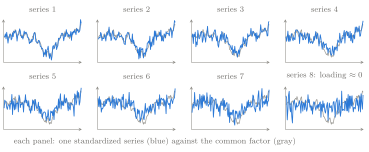
If comovement is real, then the correct response to “too many series” is not selection but aggregation with a model: treat every series as a noisy witness to a small common state, and let the model decide how much each witness’ testimony is worth. You have already seen this succeed in miniature. The Practicum 1 build combined four public weekly series into one factor and reproduced the official ten-series Weekly Economic Index with correlation 0.90. The rest of this session builds the machinery behind that result, and explains the episodes where the four-series version failed.

The first step is the smallest model in which cross-series correlation is signal rather than nuisance.

2 The Static Factor Model

2.1 One Equation, Two Kinds of Variation

Let x_\tau be an N\times1 vector of observed series for reference period \tau, each already transformed to be standardized³ and stationary. The static factor model writes each series as a linear combination of k\ll N common factors plus a series-specific remainder:

x_\tau=\Lambda f_\tau+e_\tau . \tag{1}

Read Equation 1 one object at a time. The k\times1 vector f_\tau collects the common factors: latent forces, in the sense of Session 1’s states, that many series feel at once. The N\times k matrix \Lambda holds the factor loadings; its ith row \lambda_i' says how strongly, and with what sign, series i responds to each factor. The remainder e_\tau is the idiosyncratic component: sampling error, sector-specific shocks, definitional quirks: everything in series i that is not broadly shared. “Static” refers to the equation’s form, not to the data: the factors may be highly persistent, but each period’s observation depends only on that period’s factor.

The model’s assumptions parallel Session 1’s, and it is worth stating them with the same care.

B1 (Orthogonality). Factors and idiosyncratic components are uncorrelated with each other at all leads and lags. This is what makes the split in Equation 1 meaningful: it lets every covariance between two different series be carried by the factors, and it is used each time we decompose a variance or compute a factor-extraction weight. If a “series-specific” shock in fact moves the factor, the accounting between common and idiosyncratic variation breaks down.

B2 (Weak idiosyncratic dependence). Idiosyncratic components may be correlated across series, but only weakly: no group of series shares enough leftover comovement to imitate a factor. The special case with fully uncorrelated idiosyncratics is the exact factor model; the realistic case, which tolerates limited cross-correlation, is the approximate factor model of Bai and Ng (2002). The assumption is used by every argument that averages noise away across series. It is genuinely restrictive: initial and continued unemployment claims share labor-market reporting noise that no factor should be forced to absorb, and Section 4 quantifies what such shared noise costs.

B3 (Pervasiveness). Each factor loads on a non-vanishing fraction of the series: as the panel grows, \Lambda'\Lambda/N stays bounded away from zero. This is what makes a factor recoverable from averages: a “factor” visible in only three series of a hundred cannot be separated from their idiosyncratic noise. It is used in the consistency results of Section 5.

Together, B1–B3 say what the words “common” and “idiosyncratic” mean, and they are diagnostic claims as much as conveniences: loadings and residual correlations estimated later will tell us when they are inadequate.

2.2 The Common Share

B1 makes variances add. For a standardized series i with \operatorname{Var}(f_\tau)=I_k,

\underbrace{1}_{\text{total}} =\underbrace{\lVert\lambda_i\rVert^2}_{\text{common}} +\underbrace{\sigma^2_{e,i}}_{\text{idiosyncratic}} . \tag{2}

The quantity \kappa_i=\lVert\lambda_i\rVert^2 is series i’s common share: the fraction of its variance explained by the common factors. It is the single most useful summary of an indicator’s value to a factor model. A series can be individually fascinating (much discussed, promptly released, economically interpretable) and still be nearly useless here, because most of its movement is its own.

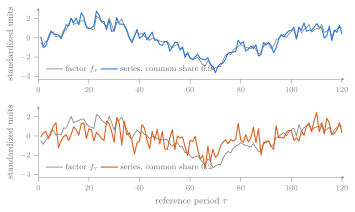
Figure 2 makes the number visible. Two series track the same factor; one has a common share of 0.9, the other 0.2. Knowing only the paths, a reader would call the first “informative” and the second “noisy,” which is exactly what the decomposition formalizes.

Figure 2: What the common share looks like. Both series load on the same factor (gray). With a common share of 0.9, the upper series is nearly a clean reading. With 0.2, the lower series contains the factor, but most of its week-to-week movement is idiosyncratic.

2.3 What the Model Says About Data

A latent-variable equation cannot be checked directly, so it is worth asking what Equation 1 implies about observable quantities. Take the covariance matrix of the panel under B1:

\Sigma =\operatorname{Var}(x_\tau) =\Lambda\Lambda'+\Psi, \qquad \Psi=\operatorname{Var}(e_\tau). \tag{3}

Read Equation 3 as the model’s entire observable content. Every covariance between two different series is carried by the low-rank piece \Lambda\Lambda': for an exact factor model with one factor, \operatorname{Cov}(x_{i\tau},x_{j\tau})=\lambda_i\lambda_j for i\neq j. The factor model is therefore a restriction on a covariance matrix: the claim that N(N-1)/2 distinct cross-series covariances can be reproduced by Nk loadings. That is a strong compression for large N, and it is testable: residual covariances that the factors cannot explain are evidence against B2, in the same way that autocorrelated innovations were evidence against Session 1’s assumptions.

Table 1 collects the notation used in this session. As in Session 1, each symbol is introduced again where it does its work.

Table 1: Notation for Session 2. The state-space symbols and the vintage superscript keep their Session 1 meanings; the number of factors is written k throughout to avoid colliding with the release date r.

Symbol	Meaning
x_\tau	N\times1 vector of standardized observed series for reference period \tau
N,\ n	Number of series (cross-section) and number of time periods
f_\tau	k\times1 vector of common factors; k is the number of factors
\Lambda,\ \lambda_i'	N\times k loading matrix and its ith row
e_\tau,\ \Psi	Idiosyncratic components and their covariance matrix
\kappa_i	Common share of series i; \kappa_i=\lVert\lambda_i\rVert^2 for standardized data
A_1,\ldots,A_p,\ u_\tau,\ \Sigma_u	Factor VAR coefficients, factor shocks, and their covariance
\rho_i,\ \varepsilon_{i\tau},\ \sigma^2_i	Idiosyncratic AR(1) coefficient, shock, and shock variance
w	Cross-sectional weights applied to the panel to extract a factor
\hat\mu_1\geq\hat\mu_2\geq\cdots	Eigenvalues of the sample covariance matrix of the panel
T,R,Z,Q,H,\ \alpha_\tau	The state-space system and state vector, exactly as defined in Session 1
r	Release date defining a data vintage, exactly as in Session 1

The model now defines what a factor is. It does not yet say which factor: the same data admit many loading–factor pairs, and the next section separates what is identified from what is chosen.

3 Rotation: What the Data Cannot Decide

3.1 Scale and Sign First

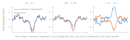
Start with one factor, because the whole problem is already visible there. If (\lambda_i, f_\tau) reproduces the data, so does (c\lambda_i,\ f_\tau/c) for any c\neq0: double every loading and halve the factor, and every product \lambda_i f_\tau is unchanged, and with it every fitted value and every covariance. Taking c=-1 flips the factor’s sign and every loading’s sign at once. Nothing observable distinguishes these representations. The factor’s scale and sign are not properties of the data; they are conventions the modeler must supply.

Figure 3 displays three of these representations. The fitted series is identical in all three panels. The “factor” is not.

Figure 3: Identical fit, different factors. The pairs (\Lambda,f), (2\Lambda,f/2), and (-\Lambda,-f) generate exactly the same observed panel. The data cannot choose among them; a normalization must.

3.2 The General Statement

With k factors the ambiguity is larger. For any invertible k\times k matrix M,

\Lambda f_\tau=(\Lambda M^{-1})(M f_\tau),

so the pair (\Lambda M^{-1},\,Mf_\tau) fits identically. The factors are identified only up to an invertible transformation: in the factor-analysis tradition, a rotation, though M need not be a rotation in the geometric sense. What is identified is the factor space: the set of linear combinations of the series that the factors span, and therefore the common component \Lambda f_\tau of each series.

This is not a defect to engineer away. It is a fact to manage with a normalization: a set of restrictions that selects one representative from each equivalence class. The standard choice, the one principal components imposes automatically, is \operatorname{Var}(f_\tau)=I_k with \Lambda'\Lambda diagonal, plus a sign convention for each factor. The Practicum 1 build’s sign rule, “the factor correlates positively with activity,” is exactly such a convention.

Two consequences deserve to be stated plainly, because both change how results are reported:

1. Factors have no intrinsic units. “The factor fell by 0.3” means nothing until the factor is scaled against something interpretable. This is why the P1 build regressed GDP growth on its factor before publishing a number, and why Section 9 treats that scaling step as part of the model.
2. Interpretation is earned, not derived. Calling the first factor “real activity” is justified by inspecting its loadings and its behavior over known episodes, not by the algebra, which would be equally satisfied by the factor’s negative.

With a normalization fixed, the model is finally specific enough to use. The natural first question is the Session 1 question: given the model’s parameters, how should the data revise our estimate of the latent factor?

4 The Factor as a Weighted Testimony

4.1 Two Witnesses, One Update

Take the smallest interesting case: one factor, two standardized series, and loadings treated as known. Let

f\sim\mathcal N(0,1), \qquad x_i=\lambda_i f+e_i, \quad \lambda_1=\lambda_2=0.8, \quad \sigma^2_{e,1}=\sigma^2_{e,2}=0.36,

with independent idiosyncratic noise, so each series has common share \kappa=0.64 by Equation 2. Suppose the two series are observed at x_1=-1.5 and x_2=-0.5: one witness reports conditions well below normal, the other only mildly below.

This is a job for Session 1’s Gaussian conditioning lemma, with f in the role of the unobserved block. The joint distribution implied by the model is

\begin{pmatrix}f\\x_1\\x_2\end{pmatrix} \sim\mathcal N\!\left( \begin{pmatrix}0\\0\\0\end{pmatrix}, \begin{pmatrix} 1&0.8&0.8\\ 0.8&1&0.64\\ 0.8&0.64&1 \end{pmatrix} \right).

The blocks come straight from Equation 3: each series has unit variance, their covariance is \lambda_1\lambda_2=0.64, and each covaries with the factor by its loading. Applying the lemma, the weight vector is w'=\Sigma_{fx}\Sigma_{xx}^{-1}, and the arithmetic gives

w_1=w_2=\tfrac{20}{41}\approx0.488, \qquad \mathbb E[f\mid x_1,x_2] =\tfrac{20}{41}(-1.5)+\tfrac{20}{41}(-0.5) =-\tfrac{40}{41}\approx-0.976, \tag{4}

with conditional variance

\operatorname{Var}(f\mid x_1,x_2) =1-w'\Sigma_{xf} =\tfrac{9}{41}\approx0.220 .

Compare the one-witness case. Observing only x_1=-1.5 gives gain \lambda_1/(\lambda_1^2+\sigma^2_{e,1})=0.8, hence \mathbb E[f\mid x_1]=-1.2 and conditional variance 0.36. The second witness did two things. It pulled the estimate up, from -1.2 to -0.976, because its milder reading is evidence that part of the first series’ plunge was idiosyncratic. And it cut the conditional variance from 0.36 to 0.220: two noisy witnesses, properly weighted, are more precise than one.

4.2 The Precision View

The same update can be computed a second way, and the second way is the one that scales. With independent idiosyncratic noise the posterior precision⁴ adds one term per witness:

\operatorname{Var}(f\mid x_1,\ldots,x_N)^{-1} =1+\sum_{i=1}^{N}\frac{\lambda_i^2}{\sigma^2_{e,i}}, \qquad \mathbb E[f\mid x] =\operatorname{Var}(f\mid x)\sum_{i=1}^{N} \frac{\lambda_i}{\sigma^2_{e,i}}\,x_i . \tag{5}

Read Equation 5 as a courtroom rule. Each witness contributes information \lambda_i^2/\sigma^2_{e,i}: testimony counts for more when the witness is more exposed to the truth (large loading) and less erratic (small idiosyncratic variance). Each observed value enters the estimate weighted by \lambda_i/\sigma^2_{e,i}, so a series with a negative loading correctly enters with a negative weight, and a series with a near-zero loading is correctly ignored no matter how dramatic its movements. For the numbers above, the posterior precision is 1+2(0.64/0.36)=41/9, reproducing \operatorname{Var}=9/41 exactly.

Extraction, in other words, is a cross-sectional regression: at each date, the panel is regressed on the loadings, with each series weighted by its precision. The time dimension plays no role yet; one cross-section is one sample.

4.3 More Witnesses, and the Blessing of Dimensionality

Now let the panel grow. With N identical independent witnesses, Equation 5 gives

\operatorname{Var}(f\mid x_1,\ldots,x_N) =\frac{1}{1+N\lambda^2/\sigma^2_e} \;\longrightarrow\;0 \quad\text{as }N\to\infty .

Every additional series is another vote, its idiosyncratic error independent of the others, and the noise averages away. In a wide enough panel the factor stops being latent in any practical sense: the cross-section alone pins it down. This is the blessing of dimensionality: the reversal by which the panel’s width, the very thing that broke regression in Section 1, becomes the source of statistical power. It is also the intuition behind the consistency results for principal components in Section 5, which make the argument without assuming the loadings are known.

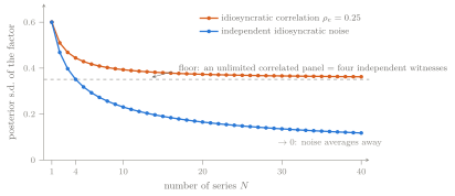
The blessing has a condition attached, and it is B2. Suppose the witnesses are not independent: each pair of idiosyncratic components shares correlation \rho_e⁵. Averaging then removes only the independent part of the noise. The average of N such witnesses has idiosyncratic variance \sigma^2_e\left[(1-\rho_e)/N+\rho_e\right]\to\sigma^2_e\rho_e, so the posterior variance no longer goes to zero:

\operatorname{Var}(f\mid x_1,\ldots,x_N) \;\longrightarrow\; \frac{1}{1+\lambda^2/(\sigma^2_e\rho_e)} \quad\text{as }N\to\infty . \tag{6}

The limit is worth restating without symbols: an unlimited supply of witnesses from one sector is worth exactly 1/\rho_e independent witnesses. With \rho_e=0.25, an infinite panel of correlated series carries the same information as four clean ones; for the anchor values \lambda=0.8, \sigma^2_e=0.36, both give posterior variance 9/73. This is the formal content of a lesson the P1 journal learned empirically: a panel of ten series from three sectors is not a ten-witness panel, and adding a fifteenth series from an already-crowded sector adds almost nothing. Boivin and Ng (2006) document the practical force of this point: larger panels assembled without regard to idiosyncratic correlation can worsen factor estimates.

Figure 4 traces both curves.

Figure 4: Why breadth beats depth. Posterior standard deviation of the factor as series are added, for the anchor values \lambda=0.8, \sigma^2_e=0.36. Independent witnesses drive uncertainty toward zero. Witnesses whose idiosyncratic noise is equicorrelated at \rho_e=0.25 hit a floor equal to four independent witnesses, no matter how many are added.

Everything in this section conditioned on known loadings. In practice \Lambda must be estimated from the same panel, and the natural estimator turns out to implement precisely this averaging logic.

5 Principal Components

5.1 The Least-Squares Problem

Stack the standardized panel as an n\times N matrix X, one row per period, one column per series. If both the loadings and the factor path are unknown, the least-squares approach chooses them to fit the panel as closely as possible:

\min_{\{\lambda_i\},\{f_\tau\}} \;\sum_{i=1}^{N}\sum_{\tau=1}^{n} \left(x_{i\tau}-\lambda_i' f_\tau\right)^2 , \tag{7}

subject to the normalization of Section 3, without which the problem has no unique solution. This is principal components in its regression form. For one factor the solution has a clean characterization: the optimal weights w form the first eigenvector⁶ of the sample covariance matrix of the panel, and the estimated factor is the weighted cross-sectional average

\hat f_\tau=w'x_\tau . \tag{8}

The derivation is one concentration step: for a fixed factor path, the best loading for each series is an ordinary regression coefficient; substituting it back turns Equation 7 into the problem of choosing the single direction in series-space that captures the most panel variance, which is what the first eigenvector is. In computation the whole object comes at once from the singular value decomposition⁷ of X: the first right singular vector is w, and the share of panel variance the factor explains is \hat\mu_1/\sum_j\hat\mu_j. Further factors, if wanted, are the subsequent eigenvectors, orthogonal by construction: the normalization \Lambda'\Lambda diagonal made real.

Notice what Equation 8 is. It is a weighted average of witnesses, with the structure of Equation 5, and with weights estimated from the panel’s own covariances rather than supplied by hand. A series that comoves strongly with the rest of the panel earns a large weight; a series that moves alone earns a weight near zero. The estimator discovers the courtroom rule.

5.2 The P1 Build as a Worked Instance

The Practicum 1 reference build runs exactly this computation on four public weekly series (each transformed and standardized; the transformation is the subject of Section 9). Its estimated weights, computed on the pre-2020 calibration sample, are worth reading like regression coefficients:

Table 2: Principal-component weights from the P1 reference build, estimated on the pre-2020 sample. The first component explains 48 percent of the calibration panel’s variance.

Series	Weight	Reading
Initial claims (sign-flipped)	0.69	High common share; carries the factor
Continued claims (sign-flipped)	0.69	High common share; carries the factor
Consumer loans	0.20	Weakly cyclical in year-over-year terms
Bank credit	−0.08	Nearly acyclical; correctly ignored

The near-zero weight on bank credit is not a failure. Banks’ balance sheets expand in panics as firms draw committed credit lines, so the series is nearly acyclical in year-over-year terms, and the estimator, seeing no comovement with the rest of the panel, correctly declines to use it. A “wrong” loading is information about the data; listen to it before deleting the series. The concentration of weight in the two claims series is also informative, and less comfortable: it says the four-series factor is mostly a labor-market factor. That observation returns with force in Section 9.

5.3 Why Averaging Works Without Knowing the Loadings

Two classical results turn principal components from a heuristic into an estimator with guarantees. First, consistency in both dimensions: as N and n grow, the estimated factor space converges to the true one, and the convergence survives the weak idiosyncratic correlation of B2 (Bai and Ng, 2002; Stock and Watson, 2002). The mechanism is the blessing of dimensionality from Section 4: each series is another noisy vote, and pervasiveness (B3) guarantees the votes keep coming. Second, a rule for choosing k: the information criteria⁸ of Bai and Ng (2002) penalize additional factors at a rate calibrated to the panel’s two dimensions, so minimizing them estimates the number of factors consistently.

Practice adds two amendments. The criteria are the referee, but parsimony is the prior: in U.S. aggregate data, one or two factors carry the business cycle, and a marginal factor tends to pick up sectoral detail: a second factor often loads on housing or finance. And no criterion substitutes for inspecting the scree plot⁹ and the loadings: a factor whose loadings have no economic pattern is usually a symptom of B2 failing, not a discovery.

5.4 What Principal Components Cannot Do

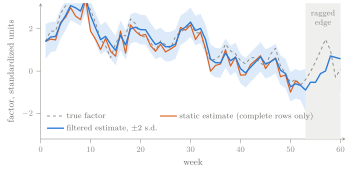
Principal components is static and complete-data, and both words are load bearing. It has no notion of factor dynamics: yesterday’s factor does not inform today’s estimate, there are no forecasts, and persistence in the data is wasted. It has no native treatment of missing observations: the SVD needs a balanced panel¹⁰, so the ragged edge, the defining feature of real-time data, forces either deleting incomplete rows or imputing them. And it produces no uncertainty bands: the factor estimate arrives without a conditional variance, so there is nothing to widen when data are thin and nothing from which to compute news weights.

All three absences point in the same direction. Dynamics, missing data, and uncertainty are exactly what Session 1’s state-space machinery provides. The factor model must be put in state space.

6 The Dynamic Factor Model

6.1 Dynamics for the Factors, and for the Noise

A dynamic factor model keeps the measurement idea of Equation 1 and adds time-series structure to both unobserved pieces:

\begin{aligned} x_\tau &= \Lambda f_\tau + e_\tau,\\ f_\tau &= A_1 f_{\tau-1}+\cdots+A_p f_{\tau-p}+u_\tau, &u_\tau&\sim\mathcal N(0,\Sigma_u),\\ e_{i\tau} &= \rho_i\,e_{i,\tau-1}+\varepsilon_{i\tau}, &\varepsilon_{i\tau}&\sim\mathcal N(0,\sigma^2_i), \end{aligned} \tag{9}

with the \varepsilon_{i\tau} independent across series. The factor equation is a vector autoregression¹¹ capturing the business cycle’s persistence: this month’s activity predicts next month’s. The idiosyncratic equations give each series’ private component its own persistence: a strike or a definitional break does not vanish in one week. Setting k=1, p=1, and \rho_i\neq0 already produces a serious nowcasting model.

Why must the idiosyncratic dynamics be modeled at all? Because Session 1’s assumptions demand it. If e_{i\tau} is serially correlated and left in the measurement error, assumption A2 (serially independent measurement noise) fails, and the filter’s innovations remain forecastable. Session 1’s discussion of that assumption already named the repair: persistence in the errors “should be modeled as additional states.” The dynamic factor model takes its own advice.

6.2 The State-Space Form

Stack the factor and every idiosyncratic component into the state. For the one-factor, first-order case,

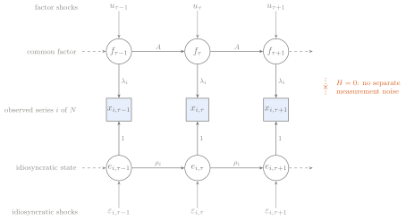
\alpha_\tau= \begin{pmatrix} f_\tau\\ e_{1\tau}\\ \vdots\\ e_{N\tau} \end{pmatrix}, \qquad T=\begin{pmatrix} a&&&\\ &\rho_1&&\\ &&\ddots&\\ &&&\rho_N \end{pmatrix}, \qquad Z=\begin{pmatrix}\Lambda & I_N\end{pmatrix}, \qquad H=0, \tag{10}

with R=I_{N+1} and Q=\operatorname{diag}(\sigma^2_u, \sigma^2_1,\ldots,\sigma^2_N). Check the dimensions before reading further: the state has N+1 elements, T is (N+1)\times(N+1) and diagonal, and Z is N\times(N+1): each measurement row picks up the factor through its loading and its own idiosyncratic state through the identity block. A factor VAR(p) replaces the single a with a kp\times kp companion block, exactly as in Session 1’s AR(p) construction.

The striking entry is H=0: the measurement equation is exact. Nothing has been swept under the rug: the measurement noise has been promoted into the state, where the filter can model its persistence instead of assuming it away. The innovations remain perfectly well defined, because uncertainty about the state still flows into every predicted observation through Z.

Once Equation 9 is written as Equation 10, everything Session 1 built applies without modification, and it is worth an explicit inventory. One forward pass of the Kalman filter now delivers:

• the factor estimate \mathbb E[f_\tau\mid Y_\tau] with a conditional variance, the uncertainty band principal components could not produce;
• forecasts of the factor, and hence of every series, through the factor VAR;
• the likelihood, evaluated from the innovations exactly as in Session 1;
• native ragged-edge handling: missing observations delete measurement rows through the selection matrix W_\tau^{(r)}, with no imputation and no deleted history; and
• mixed frequency: append monthly latent GDP growth driven by the factor, give quarterly GDP the five-weight aggregation row that Session 1 derived, and the same filter produces a quarterly GDP nowcast from a monthly panel. That combination of factor structure, the aggregation row, and ragged-edge filtering is, in structure, the nowcasting model of Giannone et al. (2008).

Figure 5 draws the dependence structure. Compare it with Session 1’s state-space graph: the new feature is that what was a single measurement-error arrow is now a persistent chain of its own inside the state.

Figure 5: The dynamic factor model as a state-space system. The common factor (top chain) and each idiosyncratic component (lower chains) evolve as persistent states. Each observed series combines the factor, through its loading, with its own idiosyncratic state. The measurement equation is exact: H=0 because all noise now lives in the state.

One practical warning belongs next to the elegance. The state has N+kp elements and the filter’s cost grows with the cube of the state dimension, so carrying every idiosyncratic component of a 130-series panel through Equation 10 is expensive. Production systems exploit the structure (the diagonal blocks in T, or sequential univariate processing of the measurement rows) or keep only the persistent idiosyncratics in the state and leave approximately white ones in H. The modeling logic is unchanged; only the linear algebra is arranged more carefully.

The system matrices T, Z, Q now contain unknown loadings, VAR coefficients, and variances. Session 1 assumed such parameters known; a factor model for a real panel cannot.

7 Estimating the Model on a Ragged Panel

Three estimation strategies are standard. They differ in how much of the model they use, and the practical craft is knowing which is sufficient for the task at hand.

Principal components alone. Estimate \hat\Lambda and \hat f_\tau by the SVD of Section 5 and stop. Fast, transparent, and reproducible in a dozen lines, but static, balanced-panel only, and silent about uncertainty. It is the right tool for a first look, for historical analysis on complete data, and for a tracker whose weekly panel is nearly balanced. This is the Practicum 1 build.

Two-step. The two-step estimator of Doz et al. (2011) runs principal components on the balanced part of the panel to obtain \hat\Lambda and the factor path, fits the factor VAR and idiosyncratic autoregressions to those estimates by least squares, then fixes all parameters and runs the Kalman filter and smoother of Session 1 over the full ragged panel. One pass, no iteration. The first step supplies the parameters; the second supplies everything principal components lacked: bands, forecasts, ragged-edge estimates, news weights. In realistic designs the efficiency loss from not iterating is small, which is why the two-step is the workhorse of daily production systems: fast, stable, and easy to audit.

Maximum likelihood by EM. The EM estimator treats the factor path as missing data and iterates two steps until the likelihood converges: an E-step that runs the Kalman smoother to compute expected states and their second moments given the current parameters, and an M-step that re-estimates every parameter by regressions on those smoothed moments (Bańbura and Modugno, 2014; Doz et al., 2012). Each iteration weakly increases the likelihood. The estimator handles arbitrary missingness (mixed frequencies, ragged edges, series that begin late or end early) inside estimation itself, not only in filtering, and it delivers the full likelihood machinery of Session 1. The price is implementation care: convergence is monotone but can be slow, and the likelihood surface contains the rotation ridge of Section 3, so the normalization must be imposed before any parameter is interpreted. Because the model is estimated by Gaussian methods without the belief that every series is exactly Gaussian, the approach is described as quasi-maximum likelihood¹². This is the standard behind serious central-bank nowcasting systems.

Table 3: Three estimators for the dynamic factor model. Each row uses strictly more of the model than the row above and costs correspondingly more.

Strategy	Uses dynamics	Handles ragged edge	Uncertainty bands	Cost	Right tool when
Principal components	no	no	no	seconds	balanced panel, first look, simple tracker
Two-step	yes	in filtering	yes	one filter pass	daily production; parameters revised rarely
EM (quasi-ML)	yes	in estimation	yes	many smoother passes	arbitrary missingness; full-system estimation

The course follows the table downward. Practicum 1 used principal components; this session’s exercises implement the two-step on a ragged panel; the capstone uses the two-step or EM as ambition allows.

8 News, Now Operational

Session 1 derived the news decomposition in general form: a nowcast revision equals \sum_i w_iv_i, surprise times weight, release by release. In the dynamic factor model that formula stops being abstract and becomes a daily production report, because the model finally says where the weights come from. The weight on release i is built from the Kalman gain of the estimated system, and the structure of Equation 9 makes its determinants legible: a release earns a large weight when its common share is high (its surprise says a lot about the factor), when it arrives early relative to other information about the same period (there is still factor uncertainty left to resolve), and when its idiosyncratic variance is small (the surprise is unlikely to be private noise).

That reading turns the decomposition into a design tool as well as a reporting tool. If the weekly claims release dominates every news report, that is not an accident of the week; it is the model reporting that claims combine high common share with first-in-the-week timing. And the caution from Session 1 carries over with more force: the model’s expectation is not the survey consensus. A release can beat the consensus and still fall short of the model’s forecast, in which case a correct news report says the release lowered the nowcast. A production commentary must say which expectation defines its surprises.

With estimation and news in place, the machinery is complete. What remains is the published object this session has been circling: the weekly tracker.

9 Anatomy of a Weekly Tracker

Lewis et al. (2022) is the cleanest published specimen of a weekly economic tracker: the Weekly Economic Index (WEI), updated every Thursday and now published by the Federal Reserve Bank of Dallas. It is the course’s replication target because every design choice in it is visible, small enough to rebuild, and instructive when it fails. Four choices define it.

9.1 Choice 1: Ten Series, Five Sectors

Table 4: The ten weekly inputs of the Weekly Economic Index, grouped by sector (Lewis et al., 2022).

Sector	Series
Labor	Initial claims; continued claims; staffing index
Consumption	Redbook same-store retail sales; consumer confidence
Production	Raw steel production; electricity output
Shipping and energy	Rail carloads; fuel sales
Taxes	Federal tax withholding

Breadth across sectors is the design principle, and Section 4 says why: series within a sector share idiosyncratic noise, so a second sector buys more precision than a fifth series from the first. The P1 build is the controlled demonstration. Its four series span only labor and credit, and its factor is, by Table 2, essentially a claims factor. On the common sample it still tracks the WEI at correlation 0.90; the blessing of dimensionality is generous. But its single largest divergence, 11.4 percentage points below the WEI in the week of March 28, 2020, is exactly the week when a claims catastrophe was deeper than the economy-wide catastrophe. The official index’s retail, fuel, and electricity series pulled its reading up; the four-series panel had no other sector to consult. Breadth is variance insurance, and the premium comes due in the weeks that matter most.

9.2 Choice 2: 52-Week Differences

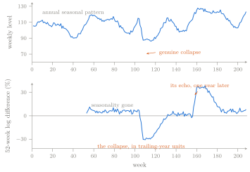
Weekly data carry ferocious seasonality: holidays, school calendars, weather, and week-ending conventions, none of it aligned across series. The WEI removes it by transformation: every input enters as its 52-week difference (in logs where appropriate),

\tilde x_{i\tau}=\ln x_{i\tau}-\ln x_{i,\tau-52}, \tag{11}

the growth of each week over the same week one year earlier. Any seasonal pattern that repeats annually cancels in the subtraction, with no seasonal model estimated and no adjustment procedure to maintain.

The price has two parts, and both are visible in Figure 6. First, the units change: the transformed series measures trailing-year growth, so the index is smoother and slower than the underlying weekly pulse: a genuine one-week collapse enters gradually and lingers. Second, every extreme week returns. Because week \tau-52 sits in the denominator of this year’s comparison, the collapse of April 2020 reappears, sign-flipped, as a spurious surge in April 2021. This is the base effect: a movement in a year-over-year series driven by the comparison week a year earlier rather than by anything current. A tracker’s user must know the difference between news and an anniversary.

Figure 6: What the 52-week difference removes, and what it costs. Top: a raw weekly series with a repeating annual pattern and a genuine mid-sample collapse. Bottom: the 52-week log difference. The seasonal pattern cancels without any model, but the collapse now enters in trailing-year units, and it echoes with the opposite sign exactly one year later, when the collapsed weeks rotate into the comparison base.

The transformation, in other words, is a seasonal adjustment in disguise: one that works only for patterns that repeat on a fixed 52-week cycle. Floating holidays drift against week numbers, and every few years a 53rd week¹³ breaks the alignment entirely. What the transformation assumes implicitly, Session 3 will model explicitly.

9.3 Choice 3: One Factor, Scaled to GDP

The WEI extracts a single principal component from the ten transformed series and then confronts the rotation problem of Section 3 head-on: a factor has no units. The solution is a scaling regression: regress four-quarter GDP growth on the quarterly-averaged factor and report the fitted value, so that a WEI reading of 2 can be read as “consistent with GDP growth of about 2 percent over the trailing year.” The P1 build does the same and estimates, on its calibration sample, \text{tracker}=2.05+0.90\times\text{factor} with a quarterly R^2 of 0.63. The regression is not decoration; it is the final, essential normalization, and it inherits every property of the sample it is fit on.

Which sample that should be is the sharpest lesson of the practicum. A coincident index standardizes its inputs and calibrates its scaling over some reference sample, and that sample choice is a modeling decision. The P1 journal’s second entry records what happens otherwise: standardizing over a sample that includes April 2020, when transformed claims sat roughly eight standard deviations from normal, inflates every standard deviation so badly that the 2008–09 recession shrinks to about one standard deviation and nearly vanishes from the fitted tracker. One episode redefined the yardstick for every other episode. The repair is a deliberate calibration window: estimate means, variances, factor weights, and the GDP scaling on a sample of normal times (the build uses pre-2020 data), then apply those fixed parameters to the full history, so that extreme episodes are measured on a normal-times yardstick rather than allowed to compress it. Every standardization has a reference population; choosing it is modeling, not housekeeping.

9.4 Choice 4: Simplicity, Deliberately

The published WEI is principal components, not a full dynamic factor model, and its maintainers know both options. The choice is instructive. A transparent index that anyone can recompute has operational value, and on a nearly balanced weekly panel the static estimator gives up little. The full state-space treatment earns its complexity when the ragged edge, uncertainty bands, or news attribution are required, which is why the same authors’ production systems, and this course’s capstone, use the machinery of Section 6. The 2020 episode forced even the simple index to adapt: the published methodology was adjusted when the pandemic’s outliers distorted the historical relationships: their production version of the standardization trap. Exercise 10 reads the published record of what changed.

Figure 7 shows the state-space payoff at the point where it matters operationally: the newest weeks of the panel, where some series have reported and others have not.

Figure 7: What the state-space form buys at the edge. Principal components requires complete rows, so its factor path ends at the last week in which every series has reported. The filtered estimate continues through the ragged edge, using whichever series have arrived, with a band that widens as the information thins.

The WEI has cousins, and knowing them frames the design space. The Chicago Fed’s CFNAI extracts one factor from 85 monthly series by principal components; it is the direct descendant of the Stock and Watson (1989) coincident index, which was the first to state the factor-plus-filter program explicitly. The ADS index of Aruoba et al. (2009) runs an exact mixed-frequency dynamic factor model on daily through quarterly data, and is closest in spirit to what this course builds. Baumeister et al. (2024) push the same design to weekly indices for each U.S. state. Between the transparent PCA tracker and the full state-space system lies most of applied nowcasting, and knowing when the simple end of the spectrum suffices is part of the craft.

10 From Comovement to a Production System

The session began with a Thursday panel that disagreed with itself. The resolution was not a better single indicator but a model of why indicators agree at all: a small number of pervasive factors, read through loadings, with everything series-specific modeled as such. It is worth an inventory of what that model now produces, because each item traces to a specific piece of machinery.

A factor estimate with a defensible weighting comes from the precision logic of Section 4, automated by principal components. An honest account of what is identified comes from Section 3, enforced by a stated normalization and a scaling regression into GDP units. Ragged-edge estimates with uncertainty bands, forecasts, a likelihood, and release-by-release news attribution come from the state-space form of Section 6 and whichever estimator in Table 3 the application justifies. And a public, reproducible weekly tracker comes from four design choices whose costs are now explicit.

What the session did not solve, it postponed deliberately, and one postponement now stands in the way. Every weekly series in this session entered through the 52-week difference, and Section 9 showed what that transformation really is: a seasonal adjustment in disguise, valid only for patterns that repeat on a fixed annual cycle, paid for in trailing-year units and anniversary echoes. High-frequency data deserve better: a model in which the seasonal pattern is estimated, can evolve, and can be separated from the signal at the data’s own frequency. What such a model looks like for weekly and even hourly data, and what “seasonally adjusted” precisely means once you must produce it yourself, is Session 3.

Exercises

Exercises marked [core] prepare material used later in the course.

Exercise 1: The covariance a factor model implies

Problem. [core, pencil] A one-factor model has three standardized series with loadings \lambda=(0.9,\,0.6,\,0.3)', factor variance 1, and mutually uncorrelated idiosyncratic components. Write the full 3\times3 covariance matrix of the observed series. Compute each series’ common share and each pairwise correlation. Which series is the most valuable witness to the factor, and what, if anything, does series 3 contribute?

TipHint

For standardized series, the diagonal entries are 1 by construction. Every off-diagonal entry must be carried by the factor: compute \operatorname{Cov}(x_i,x_j) from x_i=\lambda_i f+e_i using the orthogonality of factor and idiosyncratic components.

NoteDetailed solution

Each series is x_i=\lambda_i f+e_i with \operatorname{Var}(f)=1, \operatorname{Cov}(f,e_i)=0, and \operatorname{Cov}(e_i,e_j)=0 for i\neq j. Two facts follow directly.

For the diagonal, standardization requires 1=\lambda_i^2+\sigma^2_{e,i}, so the idiosyncratic variances are

\sigma^2_{e,1}=1-0.81=0.19, \qquad \sigma^2_{e,2}=1-0.36=0.64, \qquad \sigma^2_{e,3}=1-0.09=0.91 .

For the off-diagonals, expanding the covariance and dropping every term that orthogonality kills leaves only the factor term:

\operatorname{Cov}(x_i,x_j) =\operatorname{Cov}(\lambda_i f+e_i,\ \lambda_j f+e_j) =\lambda_i\lambda_j .

The covariance matrix, which for standardized series is also the correlation matrix, is therefore

\Sigma= \begin{pmatrix} 1&0.54&0.27\\ 0.54&1&0.18\\ 0.27&0.18&1 \end{pmatrix}.

The common shares are the squared loadings:

Series	Loading \lambda_i	Common share \lambda_i^2	Idiosyncratic share
1	0.9	0.81	0.19
2	0.6	0.36	0.64
3	0.3	0.09	0.91

Series 1 is the most valuable witness: 81 percent of its variance is factor. Series 3 is not worthless (its covariances with the other series are nonzero, and in a precision-weighted extraction it would receive a small positive weight), but 91 percent of its movement is its own story, so a large swing in series 3 alone should barely move a factor estimate.

Two checks are worth making. First, every off-diagonal has the product form \lambda_i\lambda_j; a one-factor model cannot generate any other pattern, which is what makes the model testable. Second, a common mistake is to conflate the loading with the common share: series 2’s loading of 0.6 may sound informative, but its common share is only 0.36. The loading is a correlation with the factor (for standardized data with unit factor variance), while the common share is that correlation squared.

Exercise 2: Two witnesses

Problem. [core, pencil] One factor with prior f\sim\mathcal N(0,1) is measured by two standardized series, each with loading \lambda=0.8 and idiosyncratic variance \sigma^2_e=0.36, idiosyncratic components independent. The observed values are x_1=-1.5 and x_2=-0.5. Compute the posterior mean and variance of f, twice: once by Gaussian conditioning on the joint distribution and once by precision weighting. Compare with the posterior after observing only x_1, and explain in words why the second witness pulled the estimate in the direction it did.

TipHint

Build the 3\times3 joint covariance of (f,x_1,x_2) from \operatorname{Cov}(f,x_i)=\lambda and \operatorname{Cov}(x_1,x_2)=\lambda^2, then condition. For the second route, posterior precision equals prior precision plus one term \lambda^2/\sigma^2_e per witness.

NoteDetailed solution

Route 1: joint conditioning. The model implies

\begin{pmatrix}f\\x_1\\x_2\end{pmatrix} \sim\mathcal N\!\left( \begin{pmatrix}0\\0\\0\end{pmatrix}, \begin{pmatrix} 1&0.8&0.8\\ 0.8&1&0.64\\ 0.8&0.64&1 \end{pmatrix} \right),

using \operatorname{Var}(x_i)=\lambda^2+\sigma^2_e=1 and \operatorname{Cov}(x_1,x_2)=\lambda^2=0.64. The conditioning weights are w'=\Sigma_{fx}\Sigma_{xx}^{-1}. Inverting the symmetric 2\times2 block,

\Sigma_{xx}^{-1} =\frac{1}{1-0.64^2} \begin{pmatrix}1&-0.64\\-0.64&1\end{pmatrix} =\frac{1}{0.5904} \begin{pmatrix}1&-0.64\\-0.64&1\end{pmatrix},

so each weight is

w_1=w_2=\frac{0.8(1-0.64)}{0.5904} =\frac{0.288}{0.5904} =\frac{20}{41}\approx0.488 .

The posterior mean and variance follow:

\mathbb E[f\mid x_1,x_2] =\tfrac{20}{41}(-1.5)+\tfrac{20}{41}(-0.5) =-\tfrac{40}{41}\approx-0.976,

\operatorname{Var}(f\mid x_1,x_2) =1-2\cdot\tfrac{20}{41}\cdot0.8 =1-\tfrac{32}{41} =\tfrac{9}{41}\approx0.220 .

Route 2: precision weighting. With independent idiosyncratic noise, precisions add:

\operatorname{Var}(f\mid x_1,x_2)^{-1} =1+\frac{0.64}{0.36}+\frac{0.64}{0.36} =\frac{41}{9},

reproducing \operatorname{Var}=9/41 exactly, and

\mathbb E[f\mid x_1,x_2] =\frac{9}{41}\cdot\frac{0.8}{0.36}\,(x_1+x_2) =\frac{9}{41}\cdot\frac{20}{9}\,(-2.0) =-\frac{40}{41}.

The two routes agree because they are the same projection computed in different coordinates; the precision form is the one that scales to many series.

One witness. Observing only x_1=-1.5: the gain is \lambda/(\lambda^2+\sigma^2_e)=0.8, so \mathbb E[f\mid x_1]=-1.2 and \operatorname{Var}(f\mid x_1)=1-0.8\times0.8=0.36.

The second witness moved the estimate up, from -1.2 to -0.976, while cutting the variance from 0.36 to 0.220. Both effects are informative. Series 2’s milder reading is evidence that part of series 1’s plunge was idiosyncratic rather than common; with only one witness, the model had no way to make that separation. And regardless of the values observed, a second independent witness adds precision.

A common mistake is to average the two readings to -1.0 and apply the one-series gain of 0.8, giving -0.8. That treats the average of two witnesses as if it were a single witness with the original noise level; in fact the average has idiosyncratic variance \sigma^2_e/2, which is why the correct weights differ.

Exercise 3: The witness floor

Problem. [core, pencil] N standardized series each measure a factor f\sim\mathcal N(0,1) with loading \lambda and idiosyncratic variance \sigma^2_e. Derive the posterior variance of f when the idiosyncratic components are (a) independent and (b) equicorrelated with correlation \rho_e. Show that in case (b) the posterior variance has a strictly positive limit as N\to\infty, and prove the statement: an unlimited supply of equicorrelated witnesses is worth exactly 1/\rho_e independent ones. Evaluate everything for \lambda=0.8, \sigma^2_e=0.36, \rho_e=0.25.

TipHint

By symmetry, the optimal combination of identical witnesses is their average \bar x. Work out \operatorname{Var}(\bar e) under each correlation structure, then treat \bar x=\lambda f+\bar e as a single witness.

NoteDetailed solution

Because all witnesses share the same loading and noise variance, no linear combination can beat the equally weighted average \bar x=\lambda f+\bar e, where \bar e=N^{-1}\sum_i e_i. Conditioning on \bar x is therefore equivalent to conditioning on the full vector, and a single-witness update with noise variance \operatorname{Var}(\bar e) gives the answer.

(a) Independent noise. \operatorname{Var}(\bar e)=\sigma^2_e/N, so the posterior precision is

1+\frac{\lambda^2}{\sigma^2_e/N} =1+\frac{N\lambda^2}{\sigma^2_e}, \qquad \operatorname{Var}(f\mid x_1,\ldots,x_N) =\frac{1}{1+N\lambda^2/\sigma^2_e} \;\longrightarrow\;0 .

(b) Equicorrelated noise. The average of N equicorrelated variables has variance

\operatorname{Var}(\bar e) =\frac{\sigma^2_e}{N^2} \left[N+N(N-1)\rho_e\right] =\sigma^2_e\left[\frac{1-\rho_e}{N}+\rho_e\right],

which falls with N but only to the limit \sigma^2_e\rho_e. The posterior variance is

\operatorname{Var}(f\mid x_1,\ldots,x_N) =\frac{1}{1+\dfrac{N\lambda^2}{\sigma^2_e\left[1+(N-1)\rho_e\right]}} \;\longrightarrow\; \frac{1}{1+\lambda^2/(\sigma^2_e\rho_e)}>0 .

The equivalence. In the limit, the information contributed by the panel is \lambda^2/(\sigma^2_e\rho_e)=(1/\rho_e)\cdot\lambda^2/\sigma^2_e: exactly 1/\rho_e times the information of one independent witness. An infinite equicorrelated panel therefore matches a finite independent panel of 1/\rho_e series, no more.

Numbers. With \lambda=0.8, \sigma^2_e=0.36, one witness contributes information 0.64/0.36=16/9. Independent witnesses give posterior variances

N=1:\ 0.360,\qquad N=2:\ \tfrac{9}{41}\approx0.220,\qquad N=4:\ \tfrac{9}{73}\approx0.123,\qquad N=40:\ 0.014 .

With \rho_e=0.25, the floor is

\frac{1}{1+0.64/(0.36\times0.25)} =\frac{1}{1+64/9} =\frac{9}{73}\approx0.123

which is identical to four independent witnesses, as the equivalence with 1/\rho_e=4 requires. As a finite-N check, the formula in (b) gives 0.260 at N=2 and 0.155 at N=10: the tenth correlated witness has already stopped paying.

The practical reading: a panel’s effective size is governed by its sectoral breadth, not its column count. Ten series from three sectors are closer to three witnesses than to ten, which is why adding a fifth series from an already-crowded sector is nearly free of information, the point documented empirically by Boivin and Ng (2006).

Exercise 4: Rotation, concretely

Problem. [core, pencil] (a) For a one-factor model, exhibit two loading–factor pairs besides (\Lambda,f_\tau) that generate identical data, and identify what each violates in the normalization \operatorname{Var}(f_\tau)=I, \Lambda'\Lambda diagonal, plus a sign convention. (b) For k=2, show that any pair (\Lambda M^{-1},\,Mf_\tau) with M invertible fits identically, and determine which matrices M survive the full normalization.

TipHint

For (b), impose the restrictions one at a time: which M preserve \operatorname{Var}(Mf_\tau)=I? Of those, which also keep (\Lambda M^{-1})'(\Lambda M^{-1}) diagonal with distinct diagonal entries?

NoteDetailed solution

(a) One factor. Two constructions:

• Rescaling: (2\Lambda,\ f_\tau/2). Every product \lambda_i f_\tau is unchanged, so every fitted value and every implied covariance is unchanged. It violates the variance restriction: \operatorname{Var}(f_\tau/2)=1/4\neq1.
• Sign flip: (-\Lambda,\ -f_\tau). Again all products are unchanged. It satisfies the variance restriction, since \operatorname{Var}(-f_\tau)=1, and is excluded only by the sign convention, for example “the factor correlates positively with activity.” This is why the sign convention is a necessary part of the normalization, not a nicety.

(b) Two factors. For invertible M,

(\Lambda M^{-1})(Mf_\tau)=\Lambda(M^{-1}M)f_\tau=\Lambda f_\tau ,

so the common component of every series is unchanged, and with it the entire distribution of the observed panel. Now impose the normalization on the transformed pair.

Variance restriction. \operatorname{Var}(Mf_\tau)=MM' must equal I, so M must be orthogonal: a rotation or reflection. This kills rescalings but leaves a continuum of rotations.

Diagonality restriction. Writing \tilde\Lambda=\Lambda M' (using M^{-1}=M' for orthogonal M), we need \tilde\Lambda'\tilde\Lambda=M\Lambda'\Lambda M' diagonal. If \Lambda'\Lambda is diagonal with distinct diagonal entries, the orthogonal matrices that keep it diagonal are exactly the signed permutations: reorderings of the factors combined with sign flips.

Ordering and sign conventions. Ordering the factors by explained variance removes the permutations; one sign rule per factor removes the flips. What remains is M=I: the normalization has done its job.

The edge case is instructive. If two diagonal entries of \Lambda'\Lambda are equal, so that two factors explain exactly equal variance, rotations within that two-dimensional subspace survive, and those two factors are genuinely not separately identified. In practice near-equal eigenvalues produce the near-failure: factor estimates that swap roles across samples. A common mistake in applied work is to interpret factor 2 and factor 3 of a panel separately when their eigenvalues are nearly tied; the rotation ambiguity makes the pair, not each member, the identified object.

Exercise 5: Replicate the P1 extraction

Problem. [core, computational, data] Reproduce the Practicum 1 factor extraction from scratch: pull the four weekly FRED series, transform each to a 52-week log difference with the claims series sign-flipped, standardize on the pre-2020 calibration window, and compute the first principal component of the calibration panel. Verify your weights against the reference build. Then compute each series’ common share with respect to your estimated factor and rank the four series by usefulness. Does the ranking match the weights? Should it?

TipHint

The entire extraction is one singular value decomposition of the standardized calibration panel; the weights are the first right singular vector. For the common shares, correlate each calibration-window series with the estimated factor and square.

NoteDetailed solution

The complete computation:

import io, urllib.request
import numpy as np
import pandas as pd

def fred(series_id: str) -> pd.Series:
    url = f"https://fred.stlouisfed.org/graph/fredgraph.csv?id={series_id}"
    with urllib.request.urlopen(url) as r:
        df = pd.read_csv(io.BytesIO(r.read()), na_values=".",
                         parse_dates=["observation_date"])
    return df.set_index("observation_date")[series_id].astype(float)

INPUTS = {
    "ICSA":           ("initial claims", -1),
    "CCSA":           ("continued claims", -1),
    "TOTBKCR":        ("bank credit", +1),
    "CCLACBW027SBOG": ("consumer loans", +1),
}
raw = {sid: fred(sid) for sid in INPUTS}

def yoy(s):
    w = s.resample("W-SAT").last()
    return 100 * np.log(w / w.shift(52))

panel = pd.DataFrame({name: sign * yoy(raw[sid])
                      for sid, (name, sign) in INPUTS.items()}).dropna()

CAL = panel.loc[:"2019-12-31"]          # calibration window
z   = (panel - CAL.mean()) / CAL.std()  # normal-times yardstick
zc  = z.loc[:"2019-12-31"]

U, S, Vt = np.linalg.svd(zc.values, full_matrices=False)
w = Vt[0]
factor = pd.Series(z.values @ w, index=z.index)
if factor.corr(z["initial claims"]) < 0:   # sign convention
    factor, w = -factor, -w

weights = pd.Series(w, index=z.columns)
share   = S[0]**2 / (S**2).sum()
common  = zc.corrwith(pd.Series(zc.values @ w, index=zc.index))**2

# verification against the reference build (tolerances absorb data
# revisions between the build's retrieval date and yours)
np.testing.assert_allclose(
    weights[["initial claims", "continued claims"]], [0.69, 0.69], atol=0.03)
assert abs(weights["bank credit"]) < 0.15
assert 0.44 < share < 0.52

At the retrieval date used for these notes, the computation reproduces the reference build exactly: weights 0.69, 0.69, -0.08, 0.20 for initial claims, continued claims, bank credit, and consumer loans, with the first component explaining 48 percent of calibration-panel variance. The assertions are deliberately tolerant: FRED revises claims for several weeks after each release, so a later retrieval produces slightly different numbers. That is not a bug in the exercise; it is the vintage problem of Session 1, and noting your retrieval date is part of a complete answer.

The common shares, computed on the calibration window:

Series	Weight	Common share
Initial claims	0.69	0.91
Continued claims	0.69	0.91
Consumer loans	0.20	0.08
Bank credit	−0.08	0.01

The ranking by common share matches the ranking by absolute weight, and with one factor it must, approximately: both quantities are monotone in how strongly the series comoves with the factor the panel defines. (With standardized data and a single factor, the correlation between a series and the extracted factor is close to proportional to its weight; the common share is its square.) The two rankings can diverge in a multi-factor model, where a series may earn a large weight on factor 2 while having a modest overall common share.

The economics deserves the last word. The panel is effectively two witnesses, the claims pair, plus two bystanders. Exercise 3 says what that implies: the tracker’s precision is that of a small panel however many credit series are appended, and improving it requires a new sector, not a new column.

Exercise 6: State-space fluency

Problem. [core, pencil] Write the full system matrices (T,R,Q,Z,H) for a dynamic factor model with k=2 factors following a VAR(2), AR(1) idiosyncratic components, and N=5 monthly series. Give every matrix’s dimensions and the state dimension. Then, for the one-factor version of the model, explain where the five-weight quarterly aggregation row for GDP enters and exactly which additional states it requires.

TipHint

Stack (f_\tau', f_{\tau-1}')' in companion form for the factor VAR, then append the five idiosyncratic states. For the GDP part, write monthly latent GDP growth as loading times factor plus its own idiosyncratic term, and ask which lags the tent weights touch.

NoteDetailed solution

The k=2, VAR(2), N=5 system. The state stacks the current and lagged factor vectors and the five idiosyncratic components:

\alpha_\tau= \begin{pmatrix} f_\tau\\ f_{\tau-1}\\ e_{1\tau}\\ \vdots\\ e_{5\tau} \end{pmatrix} \in\mathbb R^{9},

with dimension kp+N=2\cdot2+5=9. The transition matrix is block diagonal: a companion block for the factor VAR and a diagonal block for the idiosyncratic autoregressions,

T= \begin{pmatrix} A_1&A_2&0\\ I_2&0&0\\ 0&0&\operatorname{diag}(\rho_1,\ldots,\rho_5) \end{pmatrix},

where A_1,A_2 are 2\times2. Shocks enter the current factor block and each idiosyncratic state, but not the lagged-factor block:

R= \begin{pmatrix} I_2&0\\ 0&0\\ 0&I_5 \end{pmatrix} \ (9\times7), \qquad Q= \begin{pmatrix} \Sigma_u&0\\ 0&\operatorname{diag}(\sigma^2_1,\ldots,\sigma^2_5) \end{pmatrix} \ (7\times7).

The measurement equation reads each series off the current factors and its own idiosyncratic state:

Z=\begin{pmatrix}\Lambda&0_{5\times2}&I_5\end{pmatrix} \ (5\times9), \qquad H=0_{5\times5},

with \Lambda the 5\times2 loading matrix. The dimensions:

Object	Dimension
\alpha_\tau	9\times1
T	9\times9
R	9\times7
Q	7\times7
Z	5\times9
H	5\times5 (zero)

The zero block in Z is the answer to a frequent confusion: the lagged factors sit in the state to drive the VAR, not to be measured; only the current factors carry loadings.

The quarterly GDP row (one-factor version). Model monthly latent GDP growth as g_\tau=\gamma f_\tau+e_{g,\tau}, with e_{g,\tau} GDP’s own idiosyncratic component. The Session 1 aggregation result maps monthly growth into quarter-on-quarter growth with the tent weights, so the GDP measurement row is

y^Q_\tau =\tfrac13 g_\tau+\tfrac23 g_{\tau-1}+g_{\tau-2} +\tfrac23 g_{\tau-3}+\tfrac13 g_{\tau-4},

observed only in quarter-ending months and, within a vintage, only after the GDP release date. Substituting g_{\tau-j}=\gamma f_{\tau-j}+e_{g,\tau-j}, the row needs the current factor and its four lags, and GDP’s idiosyncratic component and its four lags: ten states for the GDP block in the one-factor case (or, equivalently, five lags of the composite g_\tau if monthly GDP growth itself is carried as a state). The factor’s companion block must therefore be extended to five lags even if the factor VAR needs fewer, exactly as the AR example in Session 1 kept lags for the measurement equation’s benefit rather than the dynamics’.

The check worth performing on any such construction: multiply out Z\alpha_\tau symbolically and confirm it reproduces the intended measurement equation for every row, then confirm that no state needed by any measurement row is dropped by the transition. Missing lag states fail silently (the filter runs, and the nowcast is simply wrong), which is why this fluency exercise is tagged core.

Exercise 7: The two-step upgrade

Problem. [core, computational] Implement the two-step estimator on a simulated ragged panel: generate n=200 periods of a one-factor panel with N=4 series, loadings (0.9,0.8,0.6,0.3), factor AR(1) coefficient 0.9, and a ragged edge (the last three observations of series 1 and the last observation of series 2 missing). Step 1: principal components and regressions on the balanced rows. Step 2: Kalman filter and smoother over the full panel with parameters fixed. Add assertions. Where does the smoothed factor differ most from the PCA factor, and which estimate tracks the true factor better?

TipHint

Treat the idiosyncratic components as measurement noise, so the state is the scalar factor: T=\hat a, Z=\hat\Lambda, H=\operatorname{diag} (\hat\sigma^2_i), Q=1-\hat a^2. At each period, use only the rows observed that period, exactly as in Session 1’s missing-data algorithm.

NoteDetailed solution

The simplest honest two-step keeps only the factor in the state and treats idiosyncratic components as (white) measurement noise, which is adequate here because the simulated idiosyncratics are white. Step 1 estimates \hat\Lambda from PCA on the balanced rows, \hat\sigma^2_i=1-\hat \lambda_i^2, and \hat a from the factor’s first autocorrelation. Step 2 is Session 1’s filter with those parameters fixed.

import numpy as np
rng = np.random.default_rng(41)

# simulate a one-factor panel with a ragged edge
n, N = 200, 4
a_true = 0.9
lam_true = np.array([0.9, 0.8, 0.6, 0.3])
sig_e = np.sqrt(1 - lam_true**2)

f = np.zeros(n)
f[0] = rng.normal()
for t in range(1, n):
    f[t] = a_true * f[t-1] + rng.normal(scale=np.sqrt(1 - a_true**2))
x = lam_true * f[:, None] + rng.normal(scale=sig_e, size=(n, N))
x[-3:, 0] = np.nan          # series 1 reports with a three-week lag
x[-1:, 1] = np.nan          # series 2 with a one-week lag

# ---- step 1: PCA and regressions on the balanced rows
balanced = ~np.isnan(x).any(axis=1)
Xb = x[balanced]
Xb_std = (Xb - Xb.mean(0)) / Xb.std(0)
U, S, Vt = np.linalg.svd(Xb_std, full_matrices=False)
w = Vt[0]
f_pca = Xb_std @ w
if np.corrcoef(f_pca, Xb_std[:, 0])[0, 1] < 0:
    f_pca, w = -f_pca, -w
f_pca /= f_pca.std()
lam_hat  = np.array([np.cov(Xb_std[:, i], f_pca)[0, 1] for i in range(N)])
sig2_hat = np.clip(1 - lam_hat**2, 0.02, None)
a_hat    = np.corrcoef(f_pca[1:], f_pca[:-1])[0, 1]
q_hat    = 1 - a_hat**2

# ---- step 2: Kalman filter + RTS smoother over the full ragged panel
xs = (x - Xb.mean(0)) / Xb.std(0)      # calibration-window standardization
a_pred, P_pred = 0.0, 1.0
filt, pred = np.empty((n, 2)), np.empty((n, 2))
for t in range(n):
    pred[t] = a_pred, P_pred
    obs = ~np.isnan(xs[t])
    if obs.any():
        Zr, y = lam_hat[obs], xs[t, obs]
        F = np.outer(Zr, Zr) * P_pred + np.diag(sig2_hat[obs])
        K = P_pred * np.linalg.solve(F, Zr)
        a_filt = a_pred + K @ (y - Zr * a_pred)
        P_filt = (1 - K @ Zr) * P_pred
    else:
        a_filt, P_filt = a_pred, P_pred
    filt[t] = a_filt, P_filt
    a_pred, P_pred = a_hat * a_filt, a_hat**2 * P_filt + q_hat

smooth = np.empty((n, 2))
smooth[-1] = filt[-1]
for t in range(n - 2, -1, -1):
    J = filt[t, 1] * a_hat / pred[t+1, 1]
    smooth[t, 0] = filt[t, 0] + J * (smooth[t+1, 0] - pred[t+1, 0])
    smooth[t, 1] = filt[t, 1] + J**2 * (smooth[t+1, 1] - pred[t+1, 1])

assert np.corrcoef(smooth[balanced, 0], f_pca)[0, 1] > 0.95
assert filt[-1, 1] > filt[100, 1]      # band widens at the ragged edge
assert np.isfinite(smooth).all()

With the seed shown, the run produces: estimated loadings (0.89, 0.87, 0.76, 0.28) against the true (0.9, 0.8, 0.6, 0.3); \hat a=0.73 against the true 0.9 (a downward bias worth noticing: the PCA factor path contains extraction noise, which attenuates its measured autocorrelation); and three results that carry the lesson:

1. On balanced rows the two factors nearly coincide, at correlation 0.98. Where data are complete, the filter has little to add to the cross-sectional average.
2. The differences concentrate exactly where data are thin. The filtered variance is 0.099 mid-sample with all four series reporting, 0.16 when series 1 drops out, and 0.31 in the final week when series 2 is also missing. PCA produces nothing at all for those weeks; the filter produces an estimate and a widening band.
3. Against the true factor, the smoothed estimate wins: correlation 0.94 versus 0.91 for PCA. The margin is the value of the dynamics: the smoother borrows strength from adjacent periods, which the static estimator cannot.

A common implementation mistake is to advance the state between two releases that belong to the same reference period, or (the two-step-specific version) to re-standardize the panel using full-sample moments in step 2 after calibrating in step 1. Both quietly change the model between the steps. The parameters, the standardization, and the reference-period bookkeeping must all be frozen when the filter takes over.

Exercise 8: Who gets credit for the news?

Problem. [core, pencil] A one-factor nowcast has prior f\sim\mathcal N(0,\,0.5) at the start of a week. Two releases arrive: claims, with loading 0.8 and idiosyncratic variance 0.36, surprises at v_1=-1.0; credit, with loading 0.3 and idiosyncratic variance 0.91, surprises at v_2=+0.5 (both measured against the prior). Compute the factor revision and its release-by-release attribution three ways: jointly, sequentially claims-first, and sequentially credit-first. Verify all three give the same final estimate, and explain why the middle numbers differ.

TipHint

For the joint route, the weight vector is w'=P_0\Lambda'(P_0\Lambda\Lambda'+\Psi)^{-1} with P_0=0.5. For the sequential routes, each scalar update is a Session 1 release update; the posterior from the first becomes the prior for the second, and the second innovation must be recomputed against the updated prior.

NoteDetailed solution

Displayed values are rounded to four decimals; every calculation uses full precision.

Joint attribution. With \Lambda=(0.8,\,0.3)', \Psi=\operatorname{diag}(0.36,\,0.91), and P_0=0.5, the observation covariance is

\operatorname{Var} \begin{pmatrix}x_1\\x_2\end{pmatrix} =P_0\Lambda\Lambda'+\Psi =\begin{pmatrix}0.68&0.12\\0.12&0.955\end{pmatrix},

and the weight vector is

w'=P_0\Lambda'\left(P_0\Lambda\Lambda'+\Psi\right)^{-1} =(0.5732,\ 0.0850).

The attribution is

Release	Surprise v_i	Weight w_i	Contribution w_iv_i
Claims	−1.0	0.5732	−0.5732
Credit	+0.5	0.0850	+0.0425
Total revision			−0.5307

Sequential, claims first. The claims update is a scalar Session 1 update: gain P_0\lambda_1/(P_0\lambda_1^2+\sigma^2_1) =0.4/0.68=0.5882, revision 0.5882\times(-1.0)=-0.5882, posterior variance (1-0.5882\times0.8)\times0.5=0.2647. Credit’s innovation must now be recomputed against the updated prior: v_2'=0.5-0.3\times(-0.5882)=0.6765. Its gain is 0.2647\times0.3/(0.09\times0.2647+0.91)=0.0850, contributing +0.0575. Final estimate: -0.5882+0.0575=-0.5307.

Sequential, credit first. Credit’s gain against the original prior is 0.15/0.955=0.1571, contributing +0.0785. Claims’ recomputed innovation is -1.0-0.8\times0.0785=-1.0628; its update contributes -0.6092. Final estimate: 0.0785-0.6092=-0.5307.

Reconciliation. All three routes end at -0.5307: in a linear Gaussian model with fixed parameters, the posterior cannot depend on the order in which the same information is processed. But credit’s credited contribution is +0.0425 jointly, +0.0575 when processed second, and +0.0785 when processed first. The reason is shared information: the two releases both carry factor news, and whichever is processed first temporarily receives credit for the overlap. The joint attribution defines one common baseline, the pre-release information set, and splits the revision simultaneously, which is why a production news table should be computed jointly for releases arriving together rather than in an arbitrary processing order.

The magnitudes are also worth a sentence. Claims earns nearly seven times credit’s weight, for exactly the reasons the chapter’s news section names: its loading is larger (more factor content per unit of surprise) and its idiosyncratic variance smaller (a claims surprise is unlikely to be private noise). A positive credit surprise of respectable size moves this nowcast by four basis points of a standard deviation; the model has, correctly, almost no use for it.

Exercise 9: Choosing the number of factors

Problem. [data] Implement the Bai and Ng (2002) criterion IC_{p2} and validate it on a simulated panel with a known number of factors before trusting it on real data. Then download the FRED-MD monthly panel (McCracken and Ng, 2016), apply the published transformation codes, standardize, and report the chosen number of factors, the variance shares of the leading components, and an interpretation of factor 2’s largest loadings. [extra] Repeat the criterion on the pre-2020 subsample and compare.

TipHint

For a standardized n\times N panel, the mean squared residual after k factors is computable from the eigenvalues alone: V(k)=\sum_{j>k}\hat\mu_j/N. The criterion is \ln V(k)+k\frac{N+n}{Nn}\ln\min(N,n). Validate on simulated data with k=3 true factors first; if your implementation cannot recover a known answer, it has nothing to say about an unknown one.

NoteDetailed solution

The criterion. For a standardized panel Z (n\times N) with sample covariance eigenvalues \hat\mu_1\geq\hat\mu_2\geq\cdots, the sum of squared residuals after removing k principal components is the sum of the discarded eigenvalues, so

IC_{p2}(k)=\ln\!\left(\frac{1}{N}\sum_{j>k}\hat\mu_j\right) +k\,\frac{N+n}{Nn}\,\ln\bigl(\min(N,n)\bigr),

and \hat k minimizes it over k=1,\ldots,k_{\max}. The penalty term is the point of the formula: it shrinks at exactly the rate at which spurious fit accumulates in the N,n\to\infty double limit, which fixed-penalty criteria like AIC and BIC do not match.

Validation. The implementation, checked on a panel where the answer is known:

import numpy as np

def ic_p2(Z, kmax=15):
    n, N = Z.shape
    mu = np.linalg.svd(Z, compute_uv=False)**2 / n
    ics = [np.log(mu[k:].sum() / N)
           + k * (N + n) / (N * n) * np.log(min(N, n))
           for k in range(1, kmax + 1)]
    return int(np.argmin(ics)) + 1, np.array(ics)

rng = np.random.default_rng(7)
n, N, k_true = 480, 120, 3
F   = rng.normal(size=(n, k_true))
Lam = rng.normal(size=(N, k_true))
X   = F @ Lam.T + rng.normal(size=(n, N))
Z   = (X - X.mean(0)) / X.std(0)

k_hat, ics = ic_p2(Z)
assert k_hat == k_true

With the seed shown, the criterion selects \hat k=3 exactly, and the IC sequence falls steeply through k=3 and then rises, the signature of a well-separated factor structure.

FRED-MD. Download the current vintage of current.csv from the FRED-MD page, apply the transformation code in each column’s first row (log differences for most real series, second differences of logs for most prices), drop series with long missing stretches and rows with any remaining missingness, standardize, and run the same function. Report four things: the chosen \hat k; the variance share of each leading component; the date of the vintage you used (FRED-MD is revised monthly, and \hat k genuinely moves across vintages and sample choices; published applications of these criteria to FRED-MD typically select on the order of seven or eight factors); and the largest loadings of factor 2.

The interpretation step is where the exercise earns its place. In most vintages, factor 1 loads broadly on real activity (production, employment, income) while factor 2’s largest loadings concentrate in a recognizable block, commonly interest rates and spreads or the price series. Write the one-sentence interpretation factor 2’s loadings support, and then note the qualification Exercise 4 taught: if \hat\mu_2 and \hat\mu_3 are close, the individual identities of factors 2 and 3 are fragile even when the pair is well identified.

[extra] The pre-2020 comparison. Rerunning the criterion on data through 2019 typically changes the count. The pandemic months are so extreme that they can dominate several eigenvalues on the full sample: the standardization trap in eigenvalue form. Whichever count you obtain, the deliverable is the comparison and its explanation, not a single “right” number: the exercise’s point is that the number of factors is an estimate with a sample attached, not a constant of nature.

Exercise 10: WEI archaeology

Problem. [data] The published Weekly Economic Index confronted its own version of the standardization trap in 2020. Using Lewis et al. (2022), Lewis et al. (2021), and the Dallas Fed’s WEI documentation, identify what the pandemic did to the index’s estimated relationships and what its maintainers changed in response. Relate each change to the calibration-window logic of the P1 build. Then propose, in one page, the v2 design for the four-series P1 tracker that best imports the lessons.

TipHint

Follow the two estimated objects separately: the factor weights and the GDP-scaling regression. For each, ask what happens mechanically when observations fifty standard deviations from normal enter its estimation sample, and what “freezing” that object would have meant.

NoteDetailed solution

What the record shows. Three findings, each traceable to the cited sources:

1. The estimated objects. The WEI is a first principal component of ten transformed weekly series, scaled by a regression onto four-quarter GDP growth (Lewis et al., 2022). Both the weights and the scaling are estimated on historical samples: precisely the two objects the P1 build learned to calibrate deliberately.
2. What 2020 did. The pandemic’s movements were tens of standard deviations on the pre-2020 yardstick. Updating the scaling regression with such observations changes the fitted slope materially; the documented discrepancies in the index’s depth at the April 2020 trough across versions trace to exactly this parameter updating (Lewis et al., 2021). This is the standardization trap operating on a published index: an extreme episode entering an estimation sample redefines the mapping applied to every other episode.
3. What the maintainers did. Alongside the baseline index, the authors published an alternative indicator measuring changes relative to a fixed February 2020 baseline, combined using the baseline WEI weights: they froze the calibration rather than letting the pandemic re-estimate it. The production documentation also separates methodology revisions from data revisions so that users can tell which kind of change moved the index. Consult the Dallas Fed’s current WEI documentation for the present-day procedure, and record the date you accessed it: the documentation itself is a vintage.

The mapping to P1. The build’s choices are the same responses in miniature: standardization moments, factor weights, and the GDP scaling all estimated on a pre-2020 calibration window and then held fixed, so that 2020 is measured on a normal-times scale rather than allowed to compress it. What P1 lacks is what the WEI’s episode exposes: a stated policy for when the calibration window itself should ever move.

A defensible v2 design. The one-page proposal should commit to, at minimum:

• A frozen calibration window with a written amendment rule. For example: parameters are re-estimated only on a fixed schedule, never mid-episode; extreme observations (beyond a stated threshold) are excluded from any future calibration sample or handled with the outlier machinery Session 1 footnoted; every parameter change is published as a methodology revision distinct from data revisions.
• Breadth before depth. Exercise 3 quantified why the claims-dominated panel has a hard precision floor; v2 should add sectors (fuel volumes, electricity, rail) rather than more labor or credit series, accepting the data-engineering cost recorded in the P1 journal.
• Vintage honesty. Claims are revised for weeks; a v2 that claims real-time validity must reconstruct from archived vintages, as the P1 brief’s stretch goal specifies.

A complete answer also names the residual risk that no calibration policy removes: a frozen yardstick measures new episodes on old units, and if the economy’s volatility regime genuinely changes, the frozen scaling will be honestly wrong rather than silently wrong. Choosing which error to accept is the design decision; Session 6’s treatment of regime dependence picks up exactly here.

Further Reading

• Stock and Watson (2002) and Bai and Ng (2002) are the two pillars of large-panel factor econometrics. Read them for the theorems’ conditions, weak dependence and pervasiveness, which is where the practice lives.

• Boivin and Ng (2006) documents when more series make factor estimates worse; it is the empirical companion to the correlated-witness floor of Section 4.

• Doz et al. (2011) develops the two-step estimator implemented in Exercise 7; Doz et al. (2012) supplies the quasi-maximum-likelihood theory behind it.

• Bańbura and Modugno (2014) is the EM reference for arbitrary missingness patterns and the standard citation behind production nowcasting systems.

• Lewis et al. (2022) is the practicum paper; read it with the P1 build open. Wegmüller and Glocker (2023) replicates and extends it, and is a model of what a careful replication looks like.

• Giannone et al. (2008) deserves a rereading now: its model is the factor-plus-aggregation state-space system of Section 6, and it will look familiar in a way it could not have after Session 1.

Session Glossary

The glossary collects the bold technical terms introduced in this session.

Hover over any dotted-underlined glossary term to see the same definition in place.

Approximate factor model

A factor model that tolerates limited correlation among idiosyncratic components rather than requiring them to be fully uncorrelated. It is the realistic setting for macroeconomic panels, and the principal-components consistency results hold under it.

Base effect

A movement in a year-over-year growth series caused by the comparison period a year earlier rather than by anything current. After an extreme episode, its anniversary produces an echo of the opposite sign that must not be read as news.

Blessing of dimensionality

The property that adding series to a factor panel sharpens the factor estimate, because independent idiosyncratic noise averages away across the cross-section. It holds only while idiosyncratic components are weakly correlated and factors load broadly.

Calibration window

The sample deliberately chosen for estimating standardization constants, factor weights, and scaling regressions, with the fitted parameters then applied to the full history. Fixing a normal-times window prevents one extreme episode from redefining the yardstick used to measure every other episode.

Coincident index

A single series constructed to summarize the current state of aggregate activity, as distinct from a forecast of a specific future target. Its usefulness depends on stated units, a stated reference sample, and a stated release calendar.

Common share

The fraction of a series’ variance explained by the common factors rather than its idiosyncratic component. Indicators with high common shares carry the most information about aggregate activity, regardless of how interesting the series is on its own.

Comovement

The tendency of many economic series to rise and fall together over the business cycle. Factor models treat that shared variation as the signal to be extracted rather than as collinearity to be fought.

Dynamic factor model

A model in which many observed series load on a few common factors that evolve over time, with persistent idiosyncratic components modeled as additional states. In state-space form it inherits the Kalman filter’s treatment of the ragged edge, uncertainty, likelihood, and news.

EM estimator

An iterative estimator that alternates between a Kalman-smoother pass computing expected states given parameters and regressions on those smoothed moments re-estimating the parameters. Each iteration weakly raises the likelihood, and arbitrary missing-data patterns are handled inside estimation itself.

Factor loading

A coefficient connecting an observed series to a common factor. Its sign and magnitude describe how the series moves with the factor under the chosen normalization, and inspecting loadings is how a factor earns an economic interpretation.

Idiosyncratic component

The part of an observed series not explained by the common factors: sampling error, sector-specific shocks, and definitional quirks. Its persistence and its correlation across series are modeling decisions with real consequences.

Normalization

A restriction on factor scale, sign, or rotation that selects one representation from the many that fit the data identically. It makes reported factors and loadings interpretable without changing anything observable.

Principal components

The least-squares estimator of a factor model, computed from the leading eigenvectors of the panel’s sample covariance matrix. It is fast and transparent on balanced panels but supplies no dynamics, no missing-data handling, and no uncertainty bands.

Rotation

An invertible transformation of the factors paired with the offsetting transformation of the loadings. Rotated factors fit the observed data exactly as well, which is why a normalization must be imposed before factors are interpreted.

Static factor model

A representation in which each observed series equals its loadings times the current common factors plus an idiosyncratic component. It describes comovement within a period but does not specify how the factors evolve.

Two-step estimator

A procedure that estimates loadings and dynamics by principal components and regression on the balanced part of a panel, then fixes those parameters and runs the Kalman filter and smoother over the full ragged panel. It trades a small efficiency loss for speed, stability, and auditability in production.

Weekly economic tracker

A high-frequency index summarizing current aggregate activity from weekly indicators, usually one factor scaled into GDP units. Its transformation window, calibration sample, and release calendar must be stated before its readings can be interpreted as growth.

References

aruoba, S. B., diebold, F. X., & scotti, C. (2009). Real-time measurement of business conditions. Journal of Business & Economic Statistics, 27(4), 417–427.

bai, J., & ng, S. (2002). Determining the number of factors in approximate factor models. Econometrica, 70(1), 191–221.

bańbura, M., & modugno, M. (2014). Maximum likelihood estimation of factor models on datasets with arbitrary pattern of missing data. Journal of Applied Econometrics, 29(1), 133–160.

baumeister, C., leiva-león, D., & sims, E. (2024). Tracking weekly state-level economic conditions. The Review of Economics and Statistics, 106(2), 483–504.

boivin, J., & ng, S. (2006). Are more data always better for factor analysis? Journal of Econometrics, 132(1), 169–194.

burns, A. F., & mitchell, W. C. (1946). Measuring business cycles. National Bureau of Economic Research.

doz, C., giannone, D., & reichlin, L. (2011). A two-step estimator for large approximate dynamic factor models based on kalman filtering. Journal of Econometrics, 164(1), 188–205.

doz, C., giannone, D., & reichlin, L. (2012). A quasi–maximum likelihood approach for large, approximate dynamic factor models. The Review of Economics and Statistics, 94(4), 1014–1024.

giannone, D., reichlin, L., & small, D. (2008). Nowcasting: The real-time informational content of macroeconomic data. Journal of Monetary Economics, 55(4), 665–676.

lewis, D. J., mertens, K., stock, J. H., & trivedi, M. (2021). High-frequency data and a weekly economic index during the pandemic. AEA Papers and Proceedings, 111, 326–330.

lewis, D. J., mertens, K., stock, J. H., & trivedi, M. (2022). Measuring real activity using a weekly economic index. Journal of Applied Econometrics, 37(4), 667–687.

mccracken, M. W., & ng, S. (2016). FRED-MD: A monthly database for macroeconomic research. Journal of Business & Economic Statistics, 34(4), 574–589.

sargent, T. J., & sims, C. A. (1977). Business cycle modeling without pretending to have too much a priori economic theory. In New methods in business cycle research (pp. 45–109). Federal Reserve Bank of Minneapolis.

stock, J. H., & watson, M. W. (1989). New indexes of coincident and leading economic indicators. In O. J. Blanchard & S. Fischer (eds.) NBER macroeconomics annual 1989 (pp. 351–394). MIT Press.

stock, J. H., & watson, M. W. (2002). Forecasting using principal components from a large number of predictors. Journal of the American Statistical Association, 97(460), 1167–1179.

wegmüller, P., & glocker, C. (2023). US weekly economic index: Replication and extension. Journal of Applied Econometrics, 38(6), 977–985.

Footnotes

1. FRED-MD is a public, monthly-updated panel of roughly 130 monthly U.S. macroeconomic series, distributed with standard transformation codes so that factor-model results can be replicated and compared across papers.

2. The ragged edge, from Session 1, is the staircase of missing values at the end of a real-time panel caused by series being released on different schedules.

3. A standardized series has had its sample mean subtracted and been divided by its sample standard deviation, so it is measured in standard-deviation units with mean zero. Which sample supplies the mean and standard deviation turns out to matter; Section 9 returns to that choice.

4. Precision is the reciprocal of a variance. Precisions of independent sources of information add, which is why it is the natural bookkeeping unit when evidence accumulates.

5. Equicorrelation assigns the same correlation to every pair. It is the cleanest way to model a sector-wide disturbance such as reporting noise or a sectoral shock that touches every series in the group equally.

6. An eigenvector of a matrix is a direction the matrix stretches without turning; the corresponding eigenvalue is the stretch factor. For a covariance matrix, the first eigenvector is the direction of maximum variance, and its eigenvalue is the variance in that direction.

7. The singular value decomposition factors any matrix as X=USV' with orthonormal U and V and nonnegative diagonal S. The columns of V are the eigenvectors of X'X, so the first column supplies the principal-component weights, and the squared singular values are proportional to the eigenvalues \hat\mu_j.

8. An information criterion scores a model by its fit minus a penalty for its size. The Bai and Ng (2002) criteria calibrate that penalty to the double limit N,n\to\infty, which ordinary AIC- or BIC-style penalties do not handle.

9. A scree plot displays the ordered eigenvalues \hat\mu_1\geq\hat\mu_2\geq\cdots. A sharp drop after the kth eigenvalue suggests k factors; the plot is suggestive rather than decisive, which is why the formal criteria exist.

10. A balanced panel has an observation for every series in every period. Real-time panels are unbalanced by construction because of the ragged edge.

11. A vector autoregression (VAR) predicts a vector of variables from p of its own lags. It is the multivariate analogue of the AR(p) process put in companion form in Session 1.

12. A quasi-maximum likelihood estimator maximizes a likelihood written under convenient distributional assumptions that need not hold exactly. Under conditions given by Doz et al. (2012), the factor estimates remain consistent even when the Gaussian assumption is only an approximation.

13. Because 52 weeks are 364 days, calendar years contain 52 weeks and a fraction; week-numbering conventions insert a 53rd week roughly every five to six years, misaligning “the same week last year” for every series at once.