---
title: "P1 · Instructor build — the weekly tracker"
subtitle: "Four public series, one factor, GDP units"
author: "Tyler Sotomayor"
date: 2026-07-30
css: [../../../sessions/notes-ebook.css]
bibliography: ../../../sessions/01-state-space-kalman/references.bib
execute:
freeze: true
warning: false
format:
html:
include-after-body: ../../../sessions/notes-chapter.html
code-fold: show
code-tools: true
---
This is the worked benchmark for [Practicum 1](../index.qmd): a weekly economic
activity tracker in the spirit of @lewis2022weekly, built from **four public
FRED series**, scaled to GDP units, and judged against the official Weekly
Economic Index. Everything below executes top to bottom; re-rendering this page
re-pulls the data.
::: {.callout-warning}
## Vintage honesty, up front
This build uses **today's FRED data**, which is revised. Initial claims in
particular are revised every week for several weeks after first release. A
production version must pull ALFRED vintages so the tracker on date $t$ uses
only what was known on date $t$ — that is the stretch goal in the brief, and
nothing in this page's backtest should be quoted as "real-time performance."
:::
## Pull
Four weekly inputs (two labor, two credit), two official benchmarks, one
quarterly target — all from FRED's keyless CSV endpoint.
```{python}
import io, urllib.request
import numpy as np
import pandas as pd

def fred(series_id: str) -> pd.Series:
    """One series from FRED's public CSV endpoint, date-indexed."""
    url = f"https://fred.stlouisfed.org/graph/fredgraph.csv?id={series_id}"
    with urllib.request.urlopen(url) as r:
        df = pd.read_csv(io.BytesIO(r.read()), na_values=".",
                         parse_dates=["observation_date"])
    return df.set_index("observation_date")[series_id].astype(float)

INPUTS = {
    "ICSA":           ("initial claims", -1),        # countercyclical
    "CCSA":           ("continued claims", -1),      # countercyclical
    "TOTBKCR":        ("bank credit", +1),
    "CCLACBW027SBOG": ("consumer loans", +1),
}
raw  = {sid: fred(sid) for sid in INPUTS}
wei  = fred("WEI")      # official Weekly Economic Index (Lewis et al.)
gdp  = fred("GDPC1")    # real GDP, quarterly

latest = max(s.index.max() for s in raw.values())
print(f"Latest weekly observation: {latest:%Y-%m-%d}")
```
## Transform
Following Lewis et al., each input becomes a **52-week log difference** — a
year-over-year growth rate that needs no seasonal adjustment, because it
compares each week to the same week a year earlier. Claims enter negated
(rising claims = falling activity). Everything is aligned to Saturday-ended
weeks and standardized over the common sample.
```{python}
def yoy(s: pd.Series) -> pd.Series:
    w = s.resample("W-SAT").last()
    return 100 * np.log(w / w.shift(52))

panel = pd.DataFrame({
    name: sign * yoy(raw[sid])
    for sid, (name, sign) in INPUTS.items()
}).dropna()
print(f"Common sample: {panel.index.min():%Y-%m-%d} → {panel.index.max():%Y-%m-%d}"
      f"  ({len(panel)} weeks × {panel.shape[1]} series)")
```
::: {.callout-important}
## The standardization trap (found the hard way)
The obvious next step — standardize each series over the full sample — is
**wrong**, and the first draft of this build made exactly that mistake. In
April 2020 initial claims ran near eight standard deviations from normal; a
full-sample standard deviation is so inflated by those weeks that the Great
Recession shrinks to about $-1.4\sigma$ and the fitted tracker barely registers
2009 at all. The [build journal](../journal.qmd) shows the broken figure. The
fix: **calibrate on the pre-2020 sample** — means, variances, factor weights,
and the GDP scaling — then apply those fixed weights to the whole history, so
extreme episodes are *measured* on a normal-times yardstick rather than
allowed to redefine it.
:::
```{python}
CAL = panel.loc[:"2019-12-31"]                 # calibration window
z   = (panel - CAL.mean()) / CAL.std()         # normal-times yardstick
```
## Extract
The first principal component — weights estimated on the calibration window,
then applied to the full history. This is the "one number" summary of the
panel, and the static cousin of the dynamic factor model we build in Session 2.
```{python}
zc = z.loc[:"2019-12-31"]
U, S, Vt = np.linalg.svd(zc.values, full_matrices=False)
w = Vt[0]
factor = pd.Series(z.values @ w, index=z.index, name="factor")
if factor.corr(z["initial claims"]) < 0:      # sign convention: pro-cyclical
    factor, w = -factor, -w

share = S[0]**2 / (S**2).sum()
print(f"First PC explains {share:.0%} of pre-2020 panel variance")
print(pd.Series(w, index=z.columns).round(2).to_string())
```
## Scale
A factor has no units. Regress four-quarter GDP growth on the quarterly
average of the factor — again on the calibration window only — and the fitted
line converts the weekly factor into **"GDP growth over the past year, in
percent"**, the same units the WEI reports.
```{python}
gdp_yoy  = (100 * np.log(gdp / gdp.shift(4))).dropna()
f_q      = factor.resample("QS").mean()
both     = pd.concat([f_q, gdp_yoy], axis=1, keys=["f", "g"]).dropna()
cal      = both.loc[:"2019-12-31"]

b, a = np.polyfit(cal["f"], cal["g"], 1)
tracker  = a + b * factor
resid    = cal["g"] - (a + b * cal["f"])
r2       = 1 - resid.var() / cal["g"].var()
print(f"tracker = {a:.2f} + {b:.2f} × factor   (pre-2020 quarterly R² = {r2:.2f})")
```
## Judge
```{python}
#| label: fig-tracker
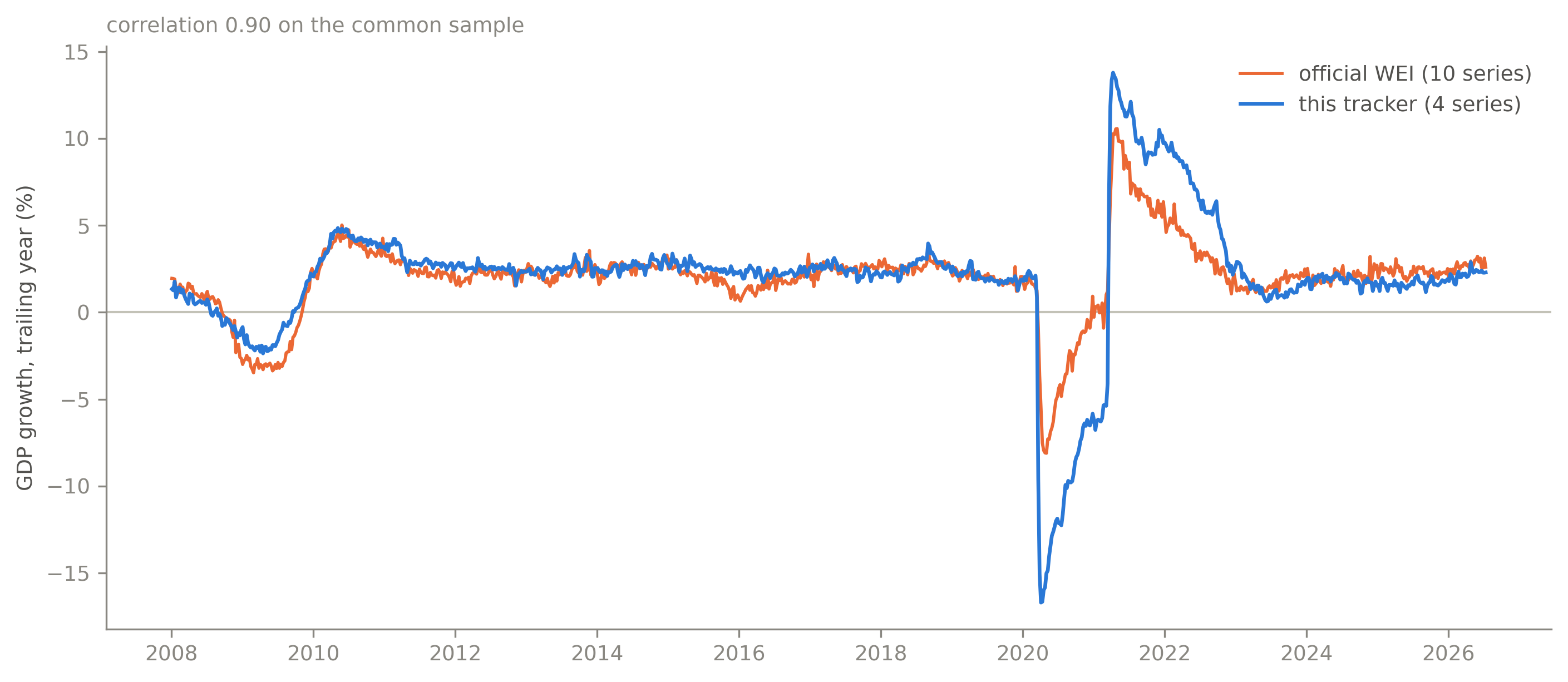
#| fig-cap: "The four-series tracker against the official ten-series WEI. One factor, public data only."
import matplotlib.pyplot as plt
INK, MUT, BLUE, ORANGE = "#52514e", "#898781", "#2a78d6", "#d9601f"
def style(ax):
for side in ("top", "right"): ax.spines[side].set_visible(False)
for side in ("left", "bottom"): ax.spines[side].set_color(MUT)
ax.tick_params(colors=MUT, labelsize=9)
ax.figure.patch.set_alpha(0); ax.patch.set_alpha(0)
common = pd.concat([tracker, wei], axis=1, keys=["ours", "wei"]).dropna()
corr = common["ours"].corr(common["wei"])
fig, ax = plt.subplots(figsize=(9.5, 4.2), dpi=150)
sub = common.loc["2008":]
ax.axhline(0, color="#c3c2b7", lw=1)
ax.plot(sub.index, sub["wei"], color=ORANGE, lw=1.4, label="official WEI (10 series)")
ax.plot(sub.index, sub["ours"], color=BLUE, lw=1.6, label="this tracker (4 series)")
ax.set_ylabel("GDP growth, trailing year (%)", color=INK, fontsize=9)
ax.legend(frameon=False, fontsize=9, labelcolor=INK)
ax.set_title(f"correlation {corr:.2f} on the common sample", loc="left",
fontsize=9, color=MUT)
style(ax); plt.tight_layout(); plt.show()
```
```{python}
#| label: fig-covid
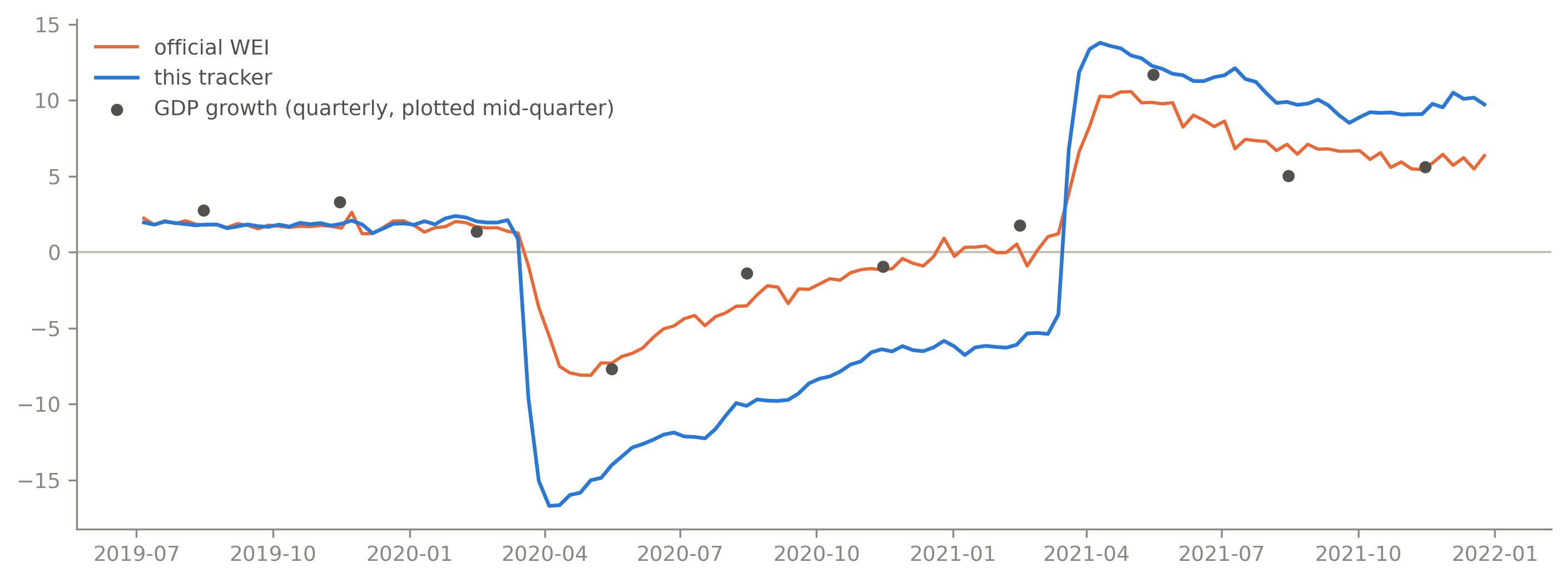
#| fig-cap: "The reason weekly trackers exist: the 2020 collapse and rebound, visible months before quarterly GDP."
fig, ax = plt.subplots(figsize=(9.5, 3.6), dpi=150)
sub = common.loc["2019-07":"2021-12"]
ax.axhline(0, color="#c3c2b7", lw=1)
ax.plot(sub.index, sub["wei"],  color=ORANGE, lw=1.4, label="official WEI")
ax.plot(sub.index, sub["ours"], color=BLUE,   lw=1.6, label="this tracker")
g = gdp_yoy.loc["2019-07":"2021-12"]
ax.scatter(g.index + pd.Timedelta(days=45), g, color=INK, s=18, zorder=5,
           label="GDP growth (quarterly, plotted mid-quarter)")
ax.legend(frameon=False, fontsize=9, labelcolor=INK)
style(ax); plt.tight_layout(); plt.show()
```
## What the comparison teaches
```{python}
#| echo: false
gap = (common["ours"] - common["wei"]).loc["2008":]
worst = gap.abs().idxmax()
print(f"Correlation with official WEI: {corr:.2f}")
print(f"Largest divergence: {worst:%Y-%m-%d} ({gap.loc[worst]:+.1f}pp)")
```
Four public series recover most of what ten curated ones deliver — that is the
factor-model promise in miniature: the business cycle is *low-dimensional*, so
a handful of noisy witnesses, properly weighted, testify to it well. The
divergences are as instructive as the agreement: our credit-heavy panel misses
sectors (retail, energy, staffing) the official WEI sees, and its largest gaps
cluster where those sectors moved independently of labor and credit. More and
better series is one fix; the Session 2 dynamic factor model — which handles
ragged edges and lets the factor have dynamics — is the other, and it is where
this course goes next.