Dynamic Factor Models

Weekly Economic Trackers — Session 2

Tyler Sotomayor · Columbia University

Thursday, 8:30, four releases

Initial claims: above the model’s expectation
Continued claims: about as expected
Bank credit, consumer loans: sideways
Session 1 says exactly how to read one of these. Which one?

Wrong question. The panel’s correlation is not a nuisance to fight — it is the signal. Today: the model built on that fact.

The oldest fact in macro: comovement

When activity turns, it turns everywhere: employment, production, sales, freight, credit — together
Burns & Mitchell (1946) built the NBER chronology on it; Sargent & Sims (1977) formalized it

The business cycle is low-dimensional. A handful of common factors — often one — drive the shared movement of everything we measure.

You’ve seen the payoff: P1’s four public series, one factor → correlation 0.90 with the official ten-series WEI.

The static factor model

x_\tau = \Lambda f_\tau + e_\tau, \qquad k \ll N

\Lambda: loadings — each series’ exposure to the common factors
e_\tau: idiosyncratic — sampling error + sector-specific movement
Standardized series split: 1 = \underbrace{\lVert\lambda_i\rVert^2}_{\text{common share}} + \sigma^2_{e,i}

A good indicator has a high common share — not an interesting personality.

What the data cannot decide

For any invertible M: \;(\Lambda M^{-1})(Mf_\tau) fits identically.

Factors identified only up to rotation, sign, scale
Managed by normalization: \operatorname{Var}(f)=I, \Lambda'\Lambda diagonal, a sign rule
Two honest consequences:
- factors have no units → scale against GDP before publishing a number
- “the activity factor” is an interpretation, earned from loadings

Reading the panel: witnesses

Two series, \lambda=0.8, noise 0.36, prior f\sim\mathcal N(0,1); observe -1.5 and -0.5:

\begin{aligned} \mathbb E[f\mid x] &= \tfrac{20}{41}(-1.5) + \tfrac{20}{41}(-0.5) = -0.98\\ \operatorname{Var}(f\mid x) &= \tfrac{9}{41} \approx 0.22 \end{aligned}

Precisions add: one witness \to variance 0.36; two \to 0.22
Weight per witness: \lambda_i/\sigma^2_{e,i} — exposure over noise
Near-zero loading \Rightarrow near-zero weight, however dramatic the series

Breadth beats depth

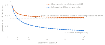
Correlated idiosyncratic noise (\rho_e) puts a floor under uncertainty: an unlimited sector = 1/\rho_e independent witnesses (Boivin–Ng 2006).

Principal components

Least squares over loadings and factors → the first eigenvector of the panel’s covariance matrix; the factor is a weighted cross-sectional average.

Consistent as N,n\to\infty, even with weak idiosyncratic correlation (Stock–Watson 2002; Bai–Ng 2002)
P1 weights, read like coefficients: claims 0.69/0.69, consumer loans 0.20, bank credit −0.08 — the estimator discovered the witness rule
Choosing k: Bai–Ng criteria referee; parsimony is the prior

What PCA cannot do → state space

PCA is static (no forecasts) and complete-data (no ragged edge), with no bands.

\begin{aligned} x_\tau &= \Lambda f_\tau + e_\tau\\ f_\tau &= A f_{\tau-1} + u_\tau, \qquad e_{i\tau} = \rho_i e_{i,\tau-1} + \varepsilon_{i\tau} \end{aligned}

State = (f_\tau, e_{1\tau},\ldots,e_{N\tau}), \;Z = (\Lambda \;\; I_N), \;H = 0 — the noise is promoted into the state (Session 1’s A2 demands it).

One Kalman pass: factor + bands · forecasts · likelihood · ragged edge natively · tent-weight GDP row → Giannone–Reichlin–Small (2008)

Estimation, three ways

PCA — fast, transparent, balanced panels (= the P1 build)
Two-step (Doz–Giannone–Reichlin 2011) — PCA for parameters, one filter/smoother pass over the ragged panel; the production workhorse (= Exercise 7)
EM / quasi-ML (Doz et al. 2012; Bańbura–Modugno 2014) — smoother ↔︎ regressions until convergence; arbitrary missingness; the central-bank standard

Course path: P1 did (1) → exercises do (2) → capstone does (2) or (3).

News, now operational

\Delta\text{nowcast} = \sum_{i\,\in\,\text{releases}} w_i \bigl(x_{i\tau} - \mathbb E[x_{i\tau}\mid\Omega_{old}]\bigr)

w_i from the estimated gain: big for high common share, early arrival, low noise
Releases arriving together: attribute jointly — sequential credit depends on processing order (Exercise 8)
The model’s surprise ≠ the consensus surprise; say which one was beaten

Anatomy of the WEI (Lewis et al. 2022)

Ten series, five sectors — breadth is variance insurance (P1’s claims-only trough: 11pp too deep in March 2020)
52-week differences — seasonal adjustment in disguise; price: trailing-year units + the base-effect echo
One factor, scaled to GDP — the normalization made useful: P1’s 2.05 + 0.90 \times factor, R^2 = 0.63
A calibration window — 2020 in the estimation sample stretches the yardstick for every other episode (the standardization trap)

Do the work

Session 2 playground — five labs in order:

two witnesses of one factor;
the witness floor;
rotation, sign, and scale;
filtering the ragged edge; and
the standardization trap.

Then the Session 2 exercises: hints and worked solutions collapse on the website; the solutions companion prints everything.

Next session

Every weekly series today entered as a 52-week difference — a seasonal adjustment in disguise, valid only for fixed annual patterns
Costs now visible: trailing-year units, anniversary echoes, floating holidays, 53-week years
Session 3: model the seasonality explicitly — STL, MSTL, TBATS, on hourly electricity load
Reading: Doz–Giannone–Reichlin (2011); reread Giannone–Reichlin–Small §3 — it will look familiar now