The Nowcasting Problem, State Space Models & the Kalman Filter

Session 1

These notes pair with the slides and the interactive Kalman filter playground. The PDF version, compiled from the same source, is under “Other Formats.”

Suppose it is 8:29 on a release morning. Our current estimate of this quarter’s GDP growth is 2.0 percent. At 8:30 a new indicator arrives below the model’s expectation. The number is relevant, but it is noisy. How far should the GDP estimate move? How much narrower should its uncertainty band become? And how can we explain the revision afterward?

Those are the questions for this session. The Kalman filter supplies the calculation, but we will not begin with the general matrix formula. We will first work through one release in a scalar model. The matrix version will then be a generalization of a calculation we already understand.

By the end of the session, you should be able to:

1. distinguish the period an observation describes from the date on which it becomes available;
2. compute a one-observation Kalman update and interpret the innovation, its variance, and the gain;
3. write a linear Gaussian state space model and run its prediction and update steps;
4. explain how missing observations and mixed frequencies enter a real-time data vintage; and
5. turn a filtered state into a quarterly GDP nowcast, an uncertainty band, and a release-by-release news decomposition.

The session assumes familiarity with matrix multiplication, transposes, variances and covariances, conditional expectation, and the multivariate normal distribution. The Gaussian conditioning result used to derive the filter is stated when we need it.

1 GDP Publication Lags, Revisions, and Nowcasting

1.1 Why GDP Must Be Estimated Before Its First Release

Real GDP is a quarterly measure. In the United States, the advance estimate is released about four weeks after a quarter ends and is revised afterward. By the middle of a quarter, the latest official GDP observation therefore describes an economy that is already several months old.

The gap matters because other decisions do not wait for the national accounts. Central banks meet, firms change production plans, and markets reprice assets while the current quarter is still under way. During that interval, evidence arrives from sources such as employment reports, industrial production, retail sales, weekly unemployment claims, electricity use, and payment data. Each indicator covers only part of the economy, and each contains noise, but together they say something about current activity.

Nowcasting is the statistical problem of using those partial measurements to estimate the present (Giannone et al., 2008). If y_Q is GDP growth in quarter Q, and \Omega_r is the information available on release date r, the nowcast is

\hat y_{Q\mid r}=\mathbb E[y_Q\mid\Omega_r]. \tag{1}

The subscript r matters. A nowcast is always attached to an information date. “Our estimate for 2027Q1” is incomplete unless we also say whether it was made in January, March, or after the quarter ended but before GDP was released.

The terminology follows the target’s position relative to the release calendar. A forecast concerns a future period. A nowcast concerns a period under way. A backcast concerns a completed period whose official value has not yet been released. In practice, the same model produces all three. Only the horizon changes.

That classification tells us which period is being estimated. It does not yet say what the forecaster was allowed to know. For that we need a second clock.

1.2 Reference Periods, Release Dates, and Data Vintages

Real-time macroeconomic data have two dates:

• The reference period, written \tau, is the week, month, or quarter the observation describes.
• The release date, written r, is the date on which that observation or revision enters the forecaster’s information set.

For example, a retail-sales number may describe July, first appear in August, and be revised in September. It belongs to July in the economic model, but it must be absent from every data vintage constructed before its August release. Neither date can replace the other.

We write x_{i,\tau}^{(r)} for the value of series i, referring to period \tau, as it appeared in vintage r. Table 1 records a small example.

Table 1: An illustrative vintage ledger. In a row such as retail sales, holding the series i=\mathrm{RS} and reference period \tau=\mathrm{Jul} fixed while moving from r_0 to r_2 traces x_{i,\tau}^{(r)} across release dates.

Series and reference period	Model notation	r_0: before release	r_1: first release	r_2: later vintage
July retail sales	x_{\mathrm{RS},\mathrm{Jul}}^{(r)}	missing	0.4%	0.2%
July industrial production	x_{\mathrm{IP},\mathrm{Jul}}^{(r)}	missing	missing	−0.1%
Previous-quarter GDP	x_{\mathrm{GDP},Q-1}^{(r)}	−1.0%	−1.0%	−0.8%

Moving from one column to the next can do two things. A previously empty cell can receive its first value, and an older value can be revised. Both events change \Omega_r. A production nowcasting system therefore stores the reference period, release timestamp, vintage value, and transformation applied to each observation.

This distinction also clarifies real-time evaluation. Using predictor values that were unavailable on date r is look-ahead bias¹. The value used later to score the nowcast is a separate choice. We may score against GDP’s first release if the objective is to predict the initial print, or against a later vintage if the objective is to estimate activity as eventually measured. Both targets can be informative, but they answer different questions.

Once the two clocks are separate, we can introduce the objects that carry information through the model. The next table is a map; the prose and examples that follow will give each symbol a job.

1.3 Notation Reference for Data Vintages, States, and Updates

Table 2 is a reference for the notation used across the session. Each symbol is introduced again where it enters the argument; there is no need to memorize the table before continuing.

Table 2: Notation used throughout Session 1.

Symbol	Meaning
\tau	Reference period of a state or observation
r	Release date, and therefore the date defining a data vintage
x_{i,\tau}^{(r)}	Value of series i for reference period \tau as available in vintage r
Y_s^{(r)}	Observations through reference period s that are available in vintage r
a_{\tau\mid s}^{(r)},\ P_{\tau\mid s}^{(r)}	Conditional mean and covariance of state \alpha_\tau given Y_s^{(r)}
W_\tau^{(r)}	Matrix selecting the observations available for period \tau in vintage r
T,R,Z	State transition, state-shock loading, and measurement loading matrices
Q,H	State-shock and measurement-error covariance matrices
Z_\tau^{(r)},\ H_\tau^{(r)}	Measurement matrix and error covariance after selecting the observed rows
T(Q),\ Z_Q	Final monthly reference period for quarter Q and the row mapping the state into quarterly GDP
v_\tau,F_\tau,K_\tau	Innovation, innovation covariance, and Kalman gain
q,\pi_\tau,\bar\pi,\bar K	Signal-to-noise ratio, scaled predicted variance, and their steady-state values in the local level model
J_\tau	Smoother gain mapping later information back to state \alpha_\tau
\tilde v_\tau	Standardized innovation used for model diagnostics

The central object is the state \alpha_\tau: a compact summary of the model at reference period \tau. The quantity a_{\tau\mid s}^{(r)} is its conditional mean², and P_{\tau\mid s}^{(r)} is its conditional covariance³. The bar in \tau\mid s can be read as “state dated \tau, given information through s.”

We now turn from the ledger to the shape it creates in a panel. Because series do not share a release schedule, the last observed reference period is not the same in every row.

1.4 Asynchronous Release Schedules and the Ragged Edge

Series are released on different schedules. On a given date, one monthly series may be available through June, another through July, and weekly claims through the previous Saturday. The lower-right corner of a data matrix is consequently incomplete. This is the ragged edge (Bańbura et al., 2011). Figure 1 shows the resulting staircase in one data vintage.

Figure 1: The ragged edge. The figure shows one vintage. Rows are ordered by publication lag, so their last available observations do not line up. GDP for the current quarter is still missing.

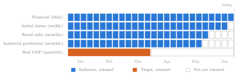
Three separate difficulties are visible here. The indicators have different frequencies, their latest observations arrive at different times, and their published histories can be revised. A statistical model can handle the first two once the vintage has been assembled correctly. It cannot recover release dates that were lost during data collection.

The data problem is now clear: information is partial, asynchronous, and revisable. To see how a model should react to one new piece of that information, we temporarily set the large panel aside and study the smallest useful update.

2 Scalar Kalman Updates in the Local Level Model

2.1 State Variation Versus Measurement Error

Before using a panel of indicators, consider one latent measure of current activity, \alpha_\tau, observed through one noisy indicator, y_\tau:

\begin{aligned} \alpha_{\tau+1} &= \alpha_\tau+\eta_\tau, & \eta_\tau&\sim\mathcal N(0,Q),\\ y_\tau &= \alpha_\tau+\varepsilon_\tau, & \varepsilon_\tau&\sim\mathcal N(0,H). \end{aligned} \tag{2}

This is the local level model. The state follows a random walk⁴. Its shock \eta_\tau allows economic conditions to change between periods. The measurement error \varepsilon_\tau represents the part of the indicator that does not measure aggregate activity: sampling error, sector-specific movements, and other idiosyncratic variation.

The distinction between Q and H is central:

• A large Q says the underlying economy can change quickly.
• A large H says the indicator is a noisy reading of that economy.

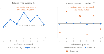
Both make observations volatile, but they imply different responses. If Q is large, recent data deserve more weight because the state may have moved. If H is large, any single observation deserves less weight because much of its movement may be measurement noise.

Figure 2 separates the two sources of volatility. Increasing Q makes the unobserved path itself less stable, so an older estimate becomes stale more quickly. Increasing H spreads observations farther around a given path, so a single reading is less trustworthy.

Figure 2: Two reasons an indicator can move. A larger Q means genuine state movement and raises the value of recent data. A larger H means a noisier reading of a given state and lowers the value of any one observation. The observed series alone cannot identify which explanation is correct without a model.

The distinction tells us qualitatively how much attention a release deserves. The next example turns that intuition into a numerical update.

2.2 Numerical Example: State Update After an Indicator Release

Return to the release morning. To keep the units interpretable, suppose the indicator has already been transformed into annualized⁵ GDP-growth units. Just before the release, the model’s distribution for current activity is

\alpha\mid\Omega_{r^-}\sim\mathcal N(a,P), \qquad a=2.0,\quad P=0.25.

Read this statement as follows: conditional on everything known just before the release, \alpha is normally distributed with center a=2.0 and variance P=0.25. The expression is a probability model for what the latent activity rate could be, not a claim that the activity rate itself is observed.

This scaling is only for the hand calculation. In an empirical model, the measurement loading Z maps an indicator in its own units into the units of the state.

The prior mean⁶ is 2.0 percent, and its standard deviation⁷ is \sqrt{0.25}=0.5 percentage points. The new indicator reads y=1.2. Its measurement-error variance is H=0.75.

The calculation has three parts. First compute the innovation, the observed release minus the model’s expectation:

v=y-a=1.2-2.0=-0.8. \tag{3}

Next compute the innovation variance and the scalar Kalman gain:

\begin{aligned} F&=P+H=1.00,\\ K&=\frac{P}{P+H}=0.25. \end{aligned} \tag{4}

Finally update the state estimate and its variance:

\begin{aligned} a^+ &= a+Kv=2.0+0.25(-0.8)=1.8,\\ P^+ &= (1-K)P=0.75(0.25)=0.1875. \end{aligned} \tag{5}

The indicator came in 0.8 percentage points below expectation. The model passes one quarter of that surprise into the state estimate, so the nowcast falls by 0.2 percentage points. The posterior standard deviation falls from 0.50 to \sqrt{0.1875}\approx0.43 because the release provided information.

This example is intentionally small, but it contains the three quantities that will recur throughout the course. Table 3 collects their numerical values and interpretations.

Table 3: The three objects in a Kalman update.

Quantity	Question it answers	Value in the example
Innovation v	How different was the release from the model’s expectation?	−0.8
Innovation variance F	How uncertain was that surprise expected to be?	1.00
Gain K	How much of the surprise should revise the state?	0.25

Two qualifications prevent common misreadings. First, K is a weight on the surprise, not on the level of the released number. Second, a release equal to its expectation has v=0, so it does not move the point estimate⁸, but it can still reduce uncertainty. Learning that an expected value actually occurred is information.

An update answers what the new release tells us about the current state. Between releases, however, the state itself continues to evolve. That requires the other half of the recursion: prediction.

2.3 State Prediction and Variance Growth Between Releases

After the update, the state moves to the next reference period according to Equation 2. Conditional on current information,

a_{\tau+1\mid\tau}=a_{\tau\mid\tau}, \qquad P_{\tau+1\mid\tau}=P_{\tau\mid\tau}+Q. \tag{6}

The mean remains unchanged because the random-walk shock has mean zero. The variance increases by Q because the next state can move before it is observed. Prediction and updating therefore have different effects: prediction adds uncertainty about state evolution; an informative observation removes some uncertainty.

Equation Equation 6 is read one line at a time. The first equality says that today’s best level is also tomorrow’s best level because the expected shock is zero. The second says that tomorrow’s uncertainty equals the uncertainty left after today’s update plus the variance of the as-yet unseen shock. The conditioning subscript \tau+1\mid\tau means “about period \tau+1, using data only through period \tau.”

For a fixed target date, the mere passage of calendar time does not reveal new information. Suppose no data arrive between Monday and Tuesday. Monday’s forecast distribution for a Friday target already allowed for the state shocks that might occur before Friday. Advancing the model one day increases the current-state variance and shortens the remaining horizon by one step; those effects offset. The target distribution changes when the information set changes, not because the clock moved.

2.4 The Signal-to-Noise Ratio and the Steady-State Kalman Gain

The numerical example used one choice of Q and H. To understand the whole family of choices, it is convenient to reduce the two variances to one relative measure. The signal-to-noise ratio compares variation in the signal⁹ with variation in the noise¹⁰:

q=\frac{Q}{H}.

Large q means that changes in the state are large relative to measurement noise. Small q means that observations are noisy relative to the pace at which the state moves. Writing the predicted variance as \pi_\tau=P_{\tau\mid\tau-1}/H, its recursion¹¹ is

\pi_{\tau+1}=\frac{\pi_\tau}{\pi_\tau+1}+q.

At a steady state¹², set \pi_{\tau+1}=\pi_\tau=\bar\pi. Then

\bar\pi=\frac{\bar\pi}{\bar\pi+1}+q \quad\Longrightarrow\quad \bar\pi(\bar\pi+1)=\bar\pi+q(\bar\pi+1) \quad\Longrightarrow\quad \bar\pi^2-q\bar\pi-q=0.

The quadratic formula gives one negative root and the positive root

\bar\pi=\frac{q+\sqrt{q^2+4q}}{2}, \qquad \bar K=\frac{\bar\pi}{\bar\pi+1}. \tag{7}

Why does the sequence reach that root? Let g(\pi)=\pi/(\pi+1)+q. For \pi\geq0, the map is increasing and

0<g'(\pi)=\frac{1}{(\pi+1)^2}\leq1.

For q>0, the inequality is strict after the first iteration. Moreover, g(\pi)-\pi is positive below \bar\pi and negative above it. An iterate therefore moves toward \bar\pi without crossing it, and each subsequent gap shrinks. The variance recursion converges to the unique nonnegative fixed point, so the gain converges to \bar K.

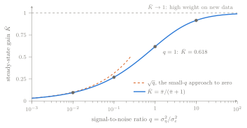
When q is large, \bar K is near one and the estimate responds strongly to new observations. When q is small, the filter averages across more observations. These statements are exact for the scalar local level model. In a multivariate system, gains can be positive or negative and depend on the full covariance structure, so it is safer to interpret them one release and one target at a time.

Figure 3 plots the steady-state gain against q. The four marked values correspond to Exercise 4.

Figure 3: Signal, noise, and the steady-state gain. A larger Q/H gives new observations more influence. The marked values correspond to Exercise 4.

2.5 Missing Observations: Prediction Without a Measurement Update

The steady-state calculation presumes regular observations. A release calendar immediately breaks that rhythm, so we next ask what the filter does when no measurement is available.

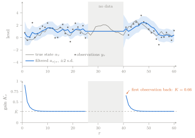
If y_\tau is missing, there is no innovation to compute. The update is skipped, and the model carries its predicted distribution forward. In the local level model, each missing period adds another Q to the state variance.

Figure 4 shows the consequences of a run of missing observations: the point estimate remains at its last updated value, uncertainty grows, and the first observation after the gap receives a larger gain.

Figure 4: A local level model during a data outage. Observations are withheld in the shaded interval. The state estimate stays at its last value while uncertainty grows. Once observations resume, the first update receives more weight because the prior is less precise.

The outage is a useful introduction to missing data, but it is not yet a full ragged edge. A real panel contains many series, and a release may describe a period earlier than the date on which it arrives. We now generalize the model while keeping those two clocks separate.

3 Linear Gaussian State-Space Models

The local level model answered one release-morning question with one state and one indicator. A production nowcast must keep track of several latent forces, their lags, and many observations at once. We therefore need notation that scales without changing the logic of the scalar calculation. This section defines that notation and states the conditions under which it has the probabilistic interpretation used later.

3.1 State and Measurement Equations: Matrices and Assumptions

A linear Gaussian¹³ state space model has two equations. The state equation describes how an m\times1 latent state vector evolves across reference periods:

\alpha_{\tau+1}=T\alpha_\tau+R\eta_\tau, \qquad \eta_\tau\sim\mathcal N(0,Q). \tag{8}

Read Equation 8 from right to left. Start with the current state \alpha_\tau, carry its predictable part forward through T, and add the new disturbance \eta_\tau through the loading matrix R. Thus T describes persistence and cross-state dynamics, while RQR' describes the uncertainty introduced on the way to \tau+1.

The measurement equation links a p\times1 observation vector to the state:

y_\tau=Z\alpha_\tau+\varepsilon_\tau, \qquad \varepsilon_\tau\sim\mathcal N(0,H). \tag{9}

Read Equation 9 as a measurement recipe. The row structure of Z converts the same state \alpha_\tau into the model’s expected value for each observed series; \varepsilon_\tau is what remains series-specific. The state equation moves through time. The measurement equation moves from an unobserved state to data at a given time.

Here T governs state dynamics, R loads shocks into the state, and Z maps the state into observed series. The covariance matrices Q and H describe state and measurement noise. Intercepts and deterministic regressors¹⁴ can be added to either equation; we omit them to keep the filtering notation readable. Any system matrix may also vary with \tau.

The assumptions used in this session are:

A1 (State noise). The sequence \{\eta_\tau\} is independent over time. This makes each \eta_\tau genuinely new state information, so the prediction variance needs only the current Q. If state shocks are serially correlated, the state must usually be enlarged to model that dependence; otherwise the filter understates what is predictable.

A2 (Measurement noise). The sequence \{\varepsilon_\tau\} is independent over time. This says that any persistence in an observed series is explained by the state rather than by leftover measurement error. If the errors are serially correlated, their dynamics should be modeled as additional states or the innovations will remain forecastable.

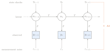
A3 (Independence). State shocks, measurement errors, and the initial state are mutually independent at all leads and lags. This removes cross-terms such as \operatorname{Cov}(R\eta_\tau,\varepsilon_{\tau+1}) from the covariance blocks used below. If economic shocks also alter reporting error, the standard gain formula is incomplete unless that covariance is included explicitly.

A4 (Initial state). \alpha_1\sim\mathcal N(a_{1\mid0},P_{1\mid0}). This supplies the distribution needed to compute the first innovation and begin the recursion. A poor but proper initialization fades as informative data arrive; a missing or internally inconsistent one leaves the first update undefined.

Together, A1, A2, A3, and A4 let means and covariances carry all information needed for the conditional distribution. The normality assumption makes those conditional distributions Gaussian. The same recursions remain best linear predictors under weaker distributional assumptions, but their interpretation as the full conditional distribution then requires care. These assumptions are therefore both conveniences and diagnostic claims: the innovations later tell us when they are inadequate.

Figure 5 displays the dependence structure implied by Equation 8, Equation 9, and assumption A3.

Figure 5: The state space model. The transition matrix T carries the state from one reference period to the next. The measurement matrix Z connects each state to observations from that period. The crossed orange path marks assumption A3: no arrow connects a state shock to a measurement error.

Within a single data vintage r, arrange the observations by reference period and write

Y_s^{(r)}=\{y_1^{(r)},\ldots,y_s^{(r)}\}.

The filtered mean¹⁵ and covariance are

a_{\tau\mid s}^{(r)} =\mathbb E[\alpha_\tau\mid Y_s^{(r)}], \qquad P_{\tau\mid s}^{(r)} =\operatorname{Var}(\alpha_\tau\mid Y_s^{(r)}). \tag{10}

The vintage superscript is essential when comparing release dates. During one filter pass it clutters every expression, so the derivation below suppresses it. The time subscripts then refer only to economic reference periods.

This notation can represent much more than an underlying level. The practical question is what the state must remember so that one step of the model contains all information needed for the next.

3.2 State Vectors for Autoregressive Lags and Model Components

The local level model uses one state. Larger states allow the model to remember lags, separate trends from cycles, and combine several common forces.

An AR(p) process¹⁶ provides a simple example. Stack the current value and its lags¹⁷, \alpha_\tau=(y_\tau,y_{\tau-1},\ldots,y_{\tau-p+1})', and use

T=\begin{pmatrix} \phi_1&\phi_2&\cdots&\phi_p\\ 1&0&\cdots&0\\ &\ddots&\ddots&\vdots\\ 0&\cdots&1&0 \end{pmatrix}, \quad R=\begin{pmatrix}1\\0\\\vdots\\0\end{pmatrix}, \quad Z=(1,0,\ldots,0).

The first row of T contains the forecasting equation. The rows underneath move each lag down one position. This companion form is the standard way to put finite-order dynamics into a first-order state equation.

The same notation will return in later sessions. Table 4 identifies the state components used by several models in the course.

Table 4: The state vector is chosen to retain the information needed for the next prediction.

Model	What the state contains	Where it returns
Local level	an underlying level	this session
Dynamic factor model	common factors and their lags	Session 2
Trend and seasonal model	level, slope, and seasonal states	Session 3
Time-varying regression	coefficients that change over time	later nonlinear and instability work

Session 2 addresses the main modeling question omitted today: when dozens of series measure activity, how should Z, the factor dynamics, and the noise covariances be estimated? For this session, take the system matrices as known while learning what the filter does with them.

4 The Multivariate Kalman Filter

The model has now separated two tasks: the state equation describes how the economy moves, and the measurement equation describes how indicators observe it. The filter combines them. Rather than present its matrix formulas as a new algorithm to memorize, we derive them from one familiar question: if two random vectors move together and one is observed, what does that observation tell us about the other?

4.1 Gaussian Derivation of the Kalman Update

The update in Equation 5 is an application of one conditional-normal formula¹⁸.

Lemma 1 (Gaussian conditioning and linear projection) If

\begin{pmatrix}x\\y\end{pmatrix} \sim\mathcal N\!\left( \begin{pmatrix}\mu_x\\\mu_y\end{pmatrix}, \begin{pmatrix} \Sigma_{xx}&\Sigma_{xy}\\ \Sigma_{yx}&\Sigma_{yy} \end{pmatrix} \right),

with \Sigma_{yy} invertible¹⁹, then

x\mid y\sim\mathcal N\!\left( \mu_x+\Sigma_{xy}\Sigma_{yy}^{-1}(y-\mu_y), \ \Sigma_{xx}-\Sigma_{xy}\Sigma_{yy}^{-1}\Sigma_{yx} \right).

Here is how to read Lemma 1. The first displayed block says that x and y are jointly normal, with their means stacked above a four-block covariance matrix. The diagonal blocks are the uncertainty in x and y separately; the off-diagonal blocks record how they move together. After y is observed, the notation x\mid y asks for the distribution of the unobserved block x conditional on that realized value.

The conditional mean has a familiar structure: prior mean plus a coefficient times a surprise. That coefficient, B=\Sigma_{xy}\Sigma_{yy}^{-1}, is the linear projection²⁰ coefficient. Indeed, the residual

u=x-\mu_x-B(y-\mu_y)

satisfies \operatorname{Cov}(u,y)=\Sigma_{xy}-B\Sigma_{yy}=0. Joint normality turns that zero covariance into independence, so observing y leaves only the residual uncertainty in u. This gives both the adjusted mean and the subtracted covariance in Lemma 1. The amount of uncertainty removed depends on the covariance structure, not on whether the realized y happens to be high or low.

The Kalman update follows once we identify x with the next state and y with its new observation. We first need their predicted joint covariance.

4.2 Matrix Prediction and Measurement-Update Equations

Suppose the current filtered distribution is

\alpha_\tau\mid Y_\tau \sim\mathcal N(a_{\tau\mid\tau},P_{\tau\mid\tau}).

The prediction step applies the state equation:

\begin{aligned} a_{\tau+1\mid\tau}&=T a_{\tau\mid\tau},\\ P_{\tau+1\mid\tau}&=T P_{\tau\mid\tau}T'+RQR'. \end{aligned} \tag{11}

Both lines follow directly from Equation 8 and the assumptions:

\begin{aligned} \mathbb E[T\alpha_\tau+R\eta_\tau\mid Y_\tau] &=T a_{\tau\mid\tau},\\ \operatorname{Var}(T\alpha_\tau+R\eta_\tau\mid Y_\tau) &=TP_{\tau\mid\tau}T'+RQR'. \end{aligned}

The first equality uses the mean-zero shock. The second propagates existing state uncertainty through T and then adds the independent uncertainty of the new shock. A covariance cross-term would appear here without A3.

Before observing y_{\tau+1}, the joint conditional distribution of state and observation is

\begin{pmatrix}\alpha_{\tau+1}\\y_{\tau+1}\end{pmatrix}\Bigm|Y_\tau \sim\mathcal N\!\left( \begin{pmatrix} a_{\tau+1\mid\tau}\\ Za_{\tau+1\mid\tau} \end{pmatrix}, \begin{pmatrix} P_{\tau+1\mid\tau}&P_{\tau+1\mid\tau}Z'\\ ZP_{\tau+1\mid\tau}&ZP_{\tau+1\mid\tau}Z'+H \end{pmatrix} \right).

Read this display as the input required by Lemma 1. The top row describes the unobserved state, the bottom row its not-yet-seen measurement. The four covariance blocks follow from the two model equations. The state has predicted covariance P_{\tau+1\mid\tau}. The observation has covariance ZP_{\tau+1\mid\tau}Z'+H: uncertainty about the state is carried through Z, and measurement noise adds H. The cross-covariance is P_{\tau+1\mid\tau}Z' because A3 makes the measurement error independent of the state.

Define the innovation and its covariance:

v_{\tau+1}=y_{\tau+1}-Za_{\tau+1\mid\tau}, \qquad F_{\tau+1}=ZP_{\tau+1\mid\tau}Z'+H. \tag{12}

In Lemma 1 set x=\alpha_{\tau+1}, y=y_{\tau+1}, \Sigma_{xy}=P_{\tau+1\mid\tau}Z', and \Sigma_{yy}=F_{\tau+1}. Substitution gives the Kalman gain and the update step:

\begin{aligned} K_{\tau+1}&=P_{\tau+1\mid\tau}Z'F_{\tau+1}^{-1},\\ a_{\tau+1\mid\tau+1} &=a_{\tau+1\mid\tau}+K_{\tau+1}v_{\tau+1},\\ P_{\tau+1\mid\tau+1} &=(I-K_{\tau+1}Z)P_{\tau+1\mid\tau}. \end{aligned} \tag{13}

Read the three lines as “weight, revise, learn.” The first line computes the weight placed on each direction of the surprise. The second adds the weighted innovation to the predicted state. The third removes the state uncertainty resolved by that observation. These are the scalar formulas from Section 2.2 with matrices in place of numbers. The gain is now an m\times p matrix. Its jth column tells us how a surprise in observation j revises each component of the state, after accounting for the covariance among all observations in that update.

The innovation has conditional mean zero²¹ and covariance F_{\tau+1}. Under the stated Gaussian assumptions²², innovations from different reference periods are independent²³. Serial correlation²⁴ in fitted innovations is therefore evidence that the model has omitted predictable structure.

4.3 Kalman Filtering with Partially Observed Data

The derivation used a complete observation vector, but the resulting recursion does not require one. At each reference period we form the same three objects from whatever rows are available. Algorithm 1 is best read as a repeated conversation between model and data: predict what should arrive, compare that prediction with what did arrive, revise, and move forward.

NoteAlgorithm 1. Kalman filter for one vintage

Start from a_{1\mid0} and P_{1\mid0}. For \tau=1,\ldots,n:

1. Form the innovation v_\tau, innovation covariance F_\tau, and gain K_\tau using the observations available for reference period \tau.
2. Update a_{\tau\mid\tau} and P_{\tau\mid\tau}. If no observation is available for that period, retain the predicted mean and covariance.
3. Predict a_{\tau+1\mid\tau} and P_{\tau+1\mid\tau}.

Store the predicted moments and innovations. They are used later for the likelihood, diagnostics, and smoother.

The stored objects matter as much as the final state. Without the predicted moments we cannot explain a release surprise, evaluate the likelihood, or run a backward smoother. Before adding the complication of a ragged panel, a short numerical pass gives us a transparent check that every stage has been coded in the intended order.

4.4 Two-Period Numerical Unit Test for the Local Level Model

Matrix notation can conceal simple timing mistakes. This example returns to the scalar model so that each number can be verified by hand and later used as a unit test for a general implementation.

Consider the local level model with Q=0.1024, H=1, a_{1\mid0}=0, and P_{1\mid0}=10. Let the first two observations be y_1=2.4 and y_2=1.9.

Table 5 applies the filter twice and records every intermediate quantity.

Table 5: Two local level filter updates. The rounded value 2.182 is used in the second innovation.

Quantity	\tau=1	\tau=2
v_\tau=y_\tau-a_{\tau\mid\tau-1}	2.400	−0.282
F_\tau=P_{\tau\mid\tau-1}+H	11.000	2.011
K_\tau=P_{\tau\mid\tau-1}/F_\tau	0.909	0.503
a_{\tau\mid\tau}	2.182	2.040
P_{\tau\mid\tau}	0.909	0.503
P_{\tau+1\mid\tau}=P_{\tau\mid\tau}+Q	1.011	0.605

The large first gain reflects the diffuse²⁵ starting variance. After the first observation, the state is much more precisely estimated, so the second release receives less weight. This table is a useful unit test for any first implementation of the filter.

4.5 Initialization and Numerically Stable Covariance Updates

Every recursion needs a place to start. In the Kalman filter, the first innovation is y_1-Za_{1\mid0} and its variance depends on P_{1\mid0}. Without an initial mean and covariance, neither quantity exists and the first release cannot be weighted. The choice of initialization says what the model knows before seeing the sample.

For a stationary state, a common choice is its unconditional mean and covariance. That choice starts the state in the same distribution implied by its long-run dynamics, so the early filter does not contain an artificial transient. After demeaning, a_{1\mid0}=0, and the covariance solves the discrete Lyapunov equation²⁶

P_{1\mid0}=TP_{1\mid0}T'+RQR'. \tag{14}

Read Equation 14 as a balance condition: the covariance before a transition must equal the covariance obtained after propagating it through T and adding one period of shock variance. A stable transition has a unique finite balance point.

For a nonstationary state such as a random walk, no unconditional covariance exists. A diffuse initialization represents weak prior information by assigning very large uncertainty to the unknown initial level. Exact diffuse methods handle the limiting case analytically; a large finite variance is a convenient approximation but should be checked for numerical sensitivity (Durbin and Koopman, 2012, ch. 5). Early diffuse periods require special treatment in the likelihood²⁷ and should usually be omitted from residual diagnostics.

Three implementation practices are worth adopting from the beginning:

1. Solve rather than invert. To obtain F_\tau^{-1}v_\tau, solve F_\tau x=v_\tau. A factorization-based solve is faster and less sensitive to rounding error than explicitly constructing an inverse.
2. Restore covariance symmetry. A true covariance satisfies P=P', but floating-point arithmetic can leave tiny asymmetric entries after many updates. Replacing P with (P+P')/2 removes that numerical artifact without changing the intended matrix.
3. Use the Joseph covariance update when needed. The Joseph covariance form²⁸ is

P_{\tau\mid\tau} =(I-K_\tau Z_\tau)P_{\tau\mid\tau-1}(I-K_\tau Z_\tau)' +K_\tau H_\tau K_\tau'. \tag{15}

With the optimal gain, Equation 15 is algebraically equivalent to the shorter covariance update. Its sum-of-quadratic-forms representation is more resistant to a computed covariance becoming indefinite. Initialization and numerical care do not change the economic model, but they determine whether the recursive calculation faithfully represents it.

5 GDP Nowcasts from Real-Time Data Vintages

The filter is now complete, but a filter is not yet a GDP nowcasting system. We still have to translate a release calendar into observed matrix rows, reconcile monthly latent growth with a quarterly target, and extract the target’s mean and variance. These are not bookkeeping details. Each step determines which economic quantity the model is estimating and which information it was allowed to use.

5.1 Observed-Row Selection for a Data Vintage

Fix a release date r. Suppose only some components²⁹ of y_\tau^{(r)} are available. Let W_\tau^{(r)} select³⁰ those components.

For example, if a three-series vector contains observations for series 1 and 3 but not series 2, then

W_\tau^{(r)} =\begin{pmatrix}1&0&0\\0&0&1\end{pmatrix}.

The measurement equation used in that vintage is

y_\tau^{obs,(r)} =W_\tau^{(r)}Z\alpha_\tau+W_\tau^{(r)}\varepsilon_\tau,

with

Z_\tau^{(r)}=W_\tau^{(r)}Z, \qquad H_\tau^{(r)}=W_\tau^{(r)}H(W_\tau^{(r)})'. \tag{16}

The first row of W_\tau^{(r)} takes the dot product with the original vector and returns its first component; the second returns its third. Multiplying Z on the left keeps the corresponding measurement rows. Multiplying H on both sides keeps their variances and the covariance between them. Equation Equation 16 is therefore the same measurement model, reduced to what could actually be observed in vintage r.

Algorithm 1 then uses only the observed rows. If a period contains no observed series, it receives a prediction step but no update.

This is computationally convenient, but it does not make the data problem trivial. The selection matrix must be built from an accurate release calendar because W_\tau^{(r)} is a claim about what was knowable on date r. If a row is included one day early, the filter uses future information; if it is included one month late or assigned to the wrong reference period, the innovation is matched to the wrong state.

A value removed after looking at its magnitude is also not automatically an innocent missing observation; that decision can introduce selection. Outliers³¹ may instead require an intervention variable³², a heavy-tailed³³ error model, or a documented rule fixed before evaluation.

When a new vintage arrives, it can fill a cell at the ragged edge or revise an older cell. The simplest reliable production procedure is to rebuild the vintage matrix and rerun the filter with fixed parameters. More specialized algorithms³⁴ can update old observations without a full pass, but they must preserve the same reference-period and release-date logic. Otherwise a computational shortcut can apply a revision to the wrong economic period or make it appear available before its actual release.

Row selection solves the “which observations?” problem. It does not yet solve the “which frequency?” problem: the state may evolve monthly while GDP is observed quarterly.

5.2 Monthly-to-Quarterly GDP Aggregation

Suppose the model runs at monthly frequency, and g_\tau is latent monthly log GDP growth. Quarterly GDP is a flow: the quarterly level is the sum of the three monthly levels. Let L_\tau be the monthly level, \ell_\tau=\log L_\tau, and g_\tau=\ell_\tau-\ell_{\tau-1}. A log-linear approximation³⁵ around three equal monthly levels gives

\log(L_\tau+L_{\tau-1}+L_{\tau-2}) \approx \log 3+\tfrac13(\ell_\tau+\ell_{\tau-1}+\ell_{\tau-2}).

Subtract the corresponding approximation for the preceding quarter:

y_\tau^Q\approx\tfrac13\left[ (\ell_\tau+\ell_{\tau-1}+\ell_{\tau-2}) -(\ell_{\tau-3}+\ell_{\tau-4}+\ell_{\tau-5})\right].

Replacing level differences with the monthly growth rates and collecting like terms yields

y_\tau^Q =\tfrac13g_\tau+\tfrac23g_{\tau-1}+g_{\tau-2} +\tfrac23g_{\tau-3}+\tfrac13g_{\tau-4}, \tag{17}

where y_\tau^Q is quarter-on-quarter log growth assigned to the final month of the quarter (Mariano and Murasawa, 2003). This is a mixed-frequency³⁶ measurement equation, not an interpolation³⁷.

If the published target is expressed at a seasonally adjusted annual rate, the model and target must be put in consistent units before estimation or reporting. Otherwise a coefficient or forecast error compares a quarterly rate with a number roughly four times as large; the model can absorb that unit error into a loading, but the reported nowcast, uncertainty, and evaluation loss will not have the intended interpretation.

Figure 6 displays the five aggregation weights. The tent shape is not a decorative pattern: it counts how many monthly levels on opposite sides of the quarterly comparison contain each growth rate. The middle growth rate affects all three month-to-month paths between the adjacent quarterly averages, while the rates at either end affect only one.

Figure 6: Monthly growth contributions to quarterly GDP growth. The middle monthly growth rate affects more terms in the comparison of adjacent quarterly averages, producing the five tent-shaped weights.

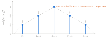
To implement Equation 17, include g_\tau and four lags in the state and give GDP the measurement row

Z_Q=(\tfrac13,\tfrac23,1,\tfrac23,\tfrac13).

Why four lags? The oldest term in Equation 17 is g_{\tau-4}. A first-order state equation can use only what its current state stores, so the vector must retain the current monthly growth rate and the four earlier rates needed by the GDP row. Fewer lags would discard a contribution before the quarterly observation could use it.

That row exists only for quarter-ending reference months. Even then, its value remains missing in vintage r until the GDP release date. This is where the two clocks matter: the observation is modeled at the quarter’s reference date but becomes available later.

The same aggregation rule does not apply to every series. Flows may be summed or averaged over a period; stocks are often measured at a point in time; rates and indexes require definitions appropriate to the series. Mixed-frequency modeling begins with those economic choices, not with a generic interpolation rule.

With the vintage rows and frequency mapping in place, the final step is to ask for the distribution of the GDP measurement implied by the filtered state.

5.3 GDP Point Nowcast and Conditional Variance

Let T(Q) denote the final monthly reference period needed to construct quarter Q. At vintage r, filter the available data through the latest reference period and predict the state to T(Q) when necessary:

\begin{aligned} a_{s+1\mid r}&=Ta_{s\mid r},\\ P_{s+1\mid r}&=TP_{s\mid r}T'+RQR'. \end{aligned} \tag{18}

Each application of Equation 18 moves the state one month closer to the quarter-ending reference period. The mean follows T; the covariance follows T and accumulates one more block of shock uncertainty RQR'.

The notation s\mid r here emphasizes that the state is dated by reference period while the conditioning information is dated by vintage. The GDP nowcast and its model-implied conditional variance are

\begin{aligned} \hat y_{Q\mid r}&=Z_Qa_{T(Q)\mid r},\\ \operatorname{Var}(y_Q\mid\Omega_r) &=Z_QP_{T(Q)\mid r}Z_Q'+H_Q. \end{aligned} \tag{19}

The first line reads the GDP target from the predicted state using the aggregation row Z_Q. The second carries state uncertainty into GDP units and adds any GDP-specific measurement variance H_Q. It is the matrix version of “estimate plus uncertainty,” evaluated for one target quarter and one release date.

As releases enter \Omega_r, the point estimate changes when their innovations are nonzero. Under a fixed linear Gaussian model with known parameters, adding observations weakly reduces the conditional variance. Calendar time without new information does not by itself narrow the band.

The variance in Equation 19 is conditional on the chosen model and its parameters. A published interval based on estimated parameters usually omits some parameter uncertainty. Bootstrap or Bayesian procedures can incorporate that additional source of uncertainty, at extra computational cost³⁸.

5.4 What the Real-Time Layer Adds

Section 5 has added three pieces around the Kalman recursion. The release calendar determines W_\tau^{(r)} and therefore which rows may update the state. The aggregation equation determines how a monthly state becomes a quarterly flow. The target row then converts the resulting state distribution into a point nowcast and uncertainty band. A correct filter applied to an incorrect calendar or frequency mapping is still an incorrect nowcast.

Those steps produce a revised number. The next question is the one a user of the nowcast will ask first: why did it change?

6 Release News and Nowcast Revisions

Operational nowcasting is not complete when the dashboard number moves. A central bank, firm, or market analyst needs to connect that revision to the releases that arrived. The same covariance calculation used by the filter gives that attribution; no second forecasting model is required.

Let \Omega_{old} be the information set before a release and \Omega_{new} the information set afterward. Let v collect the innovations in the new or revised observations, computed using the old vintage. For a target y^*, Gaussian conditioning gives

\mathbb E[y^*\mid\Omega_{new}] -\mathbb E[y^*\mid\Omega_{old}] =\operatorname{Cov}(y^*,v\mid\Omega_{old}) \operatorname{Var}(v\mid\Omega_{old})^{-1}v. \tag{20}

Write the row vector before v as w'. Then

\Delta\text{ nowcast}=\sum_i w_i v_i. \tag{21}

Each contribution has two parts:

• v_i, the difference between a release and the model’s expectation for that release;
• w_i, the way that surprise maps into the target after accounting for its precision and its covariance with the other releases.

In the scalar release from Section 2.2, v=-0.8, w=K=0.25, and the nowcast contribution is -0.2. The news decomposition³⁹ is therefore not an additional model. It records the same update in target units.

If several observations arrive together, their joint covariance belongs in the calculation. Suppose retail sales and card spending contain partly the same consumption news. A joint block recognizes that overlap and does not treat both signals as independent evidence. Sequential processing reaches the same final state in a linear model with exact arithmetic, but the first release processed temporarily receives credit for information shared with the second. Reversing the order reverses that intermediate credit. A joint block defines one common baseline and produces a simultaneous attribution that does not depend on an arbitrary ordering.

The model’s expectation is not necessarily the survey consensus quoted in a news report. A release can surprise market economists and still be close to the model’s forecast, or the reverse. A nowcast commentary should say which expectation defines its surprise.

The decomposition is exact⁴⁰ conditional⁴¹ on a fixed⁴² linear model and fixed parameters. If the model is re-estimated between vintages, part of the nowcast change comes from new parameter estimates. A complete production report should show that component separately rather than assigning it to the data releases.

Attribution assumed the system matrices were already known. To build an empirical model, we must choose them from data and then ask whether the resulting innovations behave as the model says they should.

7 Likelihood Estimation and Innovation Diagnostics

Filtering answers what the state would be if T,Z,Q,H were known. In an empirical model they are not. We need a criterion for choosing parameters and a way to check whether the fitted system has left predictable information behind. The innovation sequence supplies both: its conditional density forms the likelihood, and its standardized behavior forms the diagnostics.

7.1 Prediction-Error Likelihood for State-Space Parameters

So far, T,Z,Q,H have been treated as known. In an empirical model they contain unknown parameters \theta. The filter provides a convenient likelihood because it computes the conditional distribution of each observation given earlier observations.

The chain rule expands a joint density into successive conditional densities:

\begin{aligned} p(y_1,\ldots,y_n\mid\theta) &=p(y_n\mid Y_{n-1},\theta) p(y_{n-1}\mid Y_{n-2},\theta)\cdots p(y_1\mid\theta)\\ &=\prod_{\tau=1}^n p(y_\tau\mid Y_{\tau-1},\theta). \end{aligned}

The first line peels off the last observation, then the next-to-last, until only the first remains. The second line writes that same product compactly. The filter has already computed the mean and variance of every factor in the product, including the smaller observation blocks created by missing data.

For observed rows at period \tau, the conditional mean is Z_\tau a_{\tau\mid\tau-1}, the error is v_\tau, and its covariance is F_\tau. The Gaussian log-likelihood is

\log L(\theta) =-\frac12\sum_{\tau=1}^n \left[p_\tau\log(2\pi)+\log|F_\tau| +v_\tau'F_\tau^{-1}v_\tau\right], \tag{22}

where p_\tau is the number of observed rows. The three terms have distinct roles. The first is the normal-density constant for the observed dimension. The log determinant penalizes a model that declares a very wide predictive distribution. The quadratic form penalizes a realized innovation that is large relative to that distribution. A parameter vector fits well only by balancing calibration and sharpness.

A numerical optimizer is a search routine wrapped around the filter. It proposes a value of \theta, runs the filter, records Equation 22, and uses the change in the objective (and, when available, its derivatives) to choose a new proposal. Iteration stops when further parameter changes no longer improve the objective materially. This is useful because the state estimates depend on the parameters and the parameters’ likelihood depends on the state estimates; the optimizer closes that loop without requiring a closed-form solution.

Parameters with sign restrictions⁴³ should be transformed during optimization. If a standard deviation is written \sigma=\exp(\gamma), the optimizer may search over any real \gamma while every proposed \sigma remains positive. Without the transformation, trial steps can produce impossible covariances and make the filter fail.

Large dynamic factor models require additional identification restrictions and often use two-step⁴⁴ or EM estimators⁴⁵ Those belong in Session 2, after the factor model and its normalizations have been introduced. For now, the important point is that the innovations serve two roles: they update the state and evaluate how well a proposed parameter vector predicts the data.

A high likelihood is not proof that the model’s forecast errors have the structure we assumed. That claim has observable implications, which we check next.

7.2 Innovation Diagnostics for Bias, Scale, Dependence, and Stability

The likelihood compresses fit into one number. Diagnostics unpack it. A model can have an acceptable objective value while consistently missing in one direction, understating recession uncertainty, or leaving a lag pattern in its errors. Standardization puts innovations from different series and dates onto a common reference scale so those failures can be seen.

Under a correctly specified model, innovations have conditional mean zero and covariance F_\tau. A convenient standardized residual⁴⁶ is obtained from a matrix square root⁴⁷ such as the Cholesky factor⁴⁸ If F_\tau=L_\tau L_\tau', define

\tilde v_\tau=L_\tau^{-1}v_\tau. \tag{23}

Read Equation 23 as a solve, not as an instruction to construct L_\tau^{-1}. Compute \tilde v_\tau from L_\tau\tilde v_\tau=v_\tau. Because

\operatorname{Var}(\tilde v_\tau\mid Y_{\tau-1}) =L_\tau^{-1}F_\tau L_\tau^{-\prime}=I,

the resulting components have unit variance and no contemporaneous covariance under the model. A value of 2 now means a surprise two conditional standard deviations from zero, regardless of the original series’ units.

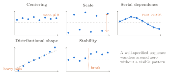
For a correctly specified linear Gaussian model, the available components of \tilde v_\tau should behave like independent standard normal draws. Useful checks include:

• Centering. A nonzero mean indicates a systematic prediction bias.
• Scale. An average squared residual far from one indicates miscalibration, but it does not identify a unique parameter at fault. The problem may involve H, Q, omitted dynamics, outliers, or instability.
• Serial dependence. Autocorrelation in residuals indicates remaining predictable structure. Autocorrelation in squared residuals suggests changing volatility.
• Distributional shape. A QQ plot reveals whether a few episodes, such as recessions or shutdowns, dominate departures from normality.
• Stability. Residual plots by date can show a model that fit one period but not another.

Figure 7 gives a stylized visual vocabulary for these checks. The panels are not test statistics; they show the kinds of patterns a statistic or plot is meant to detect.

Figure 7: What innovation failures look like. A centered, correctly scaled innovation cloud should fluctuate without pattern around zero. Each panel isolates one departure: a shifted center, excessive spread, persistent runs, unusually frequent extremes, or a relationship that changes partway through the sample.

With a ragged panel, residual dimension varies by period. Diagnostics must use the observations that were actually present, and early diffuse periods should be treated separately. Rejecting a diagnostic does not by itself prescribe the fix; it tells us what kind of model feature to investigate.

8 Filtered and Smoothed State Estimates

Filtering deliberately refuses to use the future. That is exactly right for a real-time nowcast, but it is not always the question an analyst wants to answer. After the full vintage is available, later observations may clarify whether an earlier movement was a genuine change in the state or temporary measurement noise. Smoothing passes that later information backward while keeping the vintage itself fixed.

8.1 Two Information Sets, Two Estimates

A filtered estimate respects the information available at each reference period within a vintage. A smoothed estimate asks a different question: using the entire vintage Y_n, what do we infer about an earlier state? At the last period the two coincide, because there are no later observations to add. Earlier in the sample they can differ in both their means and their uncertainty.

8.2 Deriving the Backward Recursion

Starting from the last filtered state, the Rauch–Tung–Striebel smoother runs backward. Conditional on Y_\tau, the state equation implies

\begin{aligned} \operatorname{Cov}(\alpha_\tau,\alpha_{\tau+1}\mid Y_\tau) &=P_{\tau\mid\tau}T',\\ \operatorname{Var}(\alpha_{\tau+1}\mid Y_\tau) &=P_{\tau+1\mid\tau}. \end{aligned}

Why is the backward weight covariance times inverse variance? Consider a linear prediction of the current state error from the next-state prediction error:

(\alpha_\tau-a_{\tau\mid\tau}) \approx B(\alpha_{\tau+1}-a_{\tau+1\mid\tau}).

The least-squares normal equation sets the residual uncorrelated with the predictor,

B\operatorname{Var}(\alpha_{\tau+1}\mid Y_\tau) =\operatorname{Cov}(\alpha_\tau,\alpha_{\tau+1}\mid Y_\tau).

Solving for B gives covariance times inverse variance. Substituting the two blocks above defines the smoother gain:

J_\tau=P_{\tau\mid\tau}T'P_{\tau+1\mid\tau}^{-1}.

This has the same covariance-over-variance form as the Kalman gain because both are linear projections. The filter projects a state on a contemporaneous data surprise; the smoother projects an earlier state on what we later learned about the next state. Applying Lemma 1 to \alpha_\tau and \alpha_{\tau+1}, then averaging over what the full vintage Y_n tells us about \alpha_{\tau+1}, gives the backward recursions

\begin{aligned} a_{\tau\mid n} &=a_{\tau\mid\tau} +J_\tau(a_{\tau+1\mid n}-a_{\tau+1\mid\tau}),\\ P_{\tau\mid n} &=P_{\tau\mid\tau} +J_\tau(P_{\tau+1\mid n}-P_{\tau+1\mid\tau})J_\tau'. \end{aligned} \tag{24}

Read the mean line as “filtered estimate plus backward revision.” The difference a_{\tau+1\mid n}-a_{\tau+1\mid\tau} is what later observations taught the model about the next state. The smoother gain J_\tau maps the predictable part of that news back to period \tau. In the covariance line, P_{\tau+1\mid n}-P_{\tau+1\mid\tau} is negative semidefinite because later data cannot add uncertainty about the next state; premultiplying and postmultiplying by J_\tau transfers that reduction backward.

Figure 8 compares the filtered and smoothed paths and their conditional standard deviations.

Figure 8: Filtered and smoothed estimates. The filtered path uses observations only through each date. The smoothed path uses the full simulated sample. Where later states are informative about earlier ones, the smoothed band is narrower.

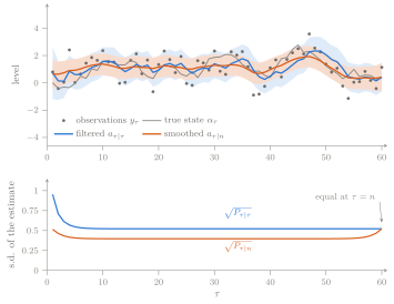
Filtered estimates are the appropriate objects for reconstructing what could have been known in real time. Smoothed estimates are useful for historical description and for parameter-estimation procedures such as EM. Smoothing cannot increase conditional variance, although it may leave it unchanged when future observations contain no information about a particular earlier state.

That distinction matters directly for evaluation. A historical smoothed path may be the best retrospective account of the economy, but using it as though it were available at an earlier forecast origin would reintroduce look-ahead bias.

9 Real-Time Backtesting with GDP Vintages

The purpose of evaluation is not merely to rank two RMSEs. It is to learn when a model adds information, how that conclusion depends on the target vintage and horizon, and how uncertain the apparent advantage is. A credible design must recreate the decision problem the forecaster actually faced.

9.1 Replaying the Information Set

A credible backtest replays the information flow. Choose a sequence of forecast origins r. At each origin:

1. build the vintage containing only values available by r;
2. apply transformations using information available by r;
3. estimate or fix parameters according to a rule chosen in advance;
4. produce and store the nowcast and its uncertainty; and
5. record the horizon relative to the target’s release date.

This produces an accuracy profile by horizon, not just one error statistic. A model may be useful early in the quarter and add little near the GDP release, or the reverse.

The parameter rule in step 3 is part of the experiment. Expanding-window estimation mimics a model re-estimated using all history available at each origin; fixed-parameter evaluation isolates filtering performance but gives the historical forecaster parameter knowledge it may not have had. Either can be useful if it is labeled. Silently mixing the two makes the comparison irreproducible.

9.2 Targets, Losses, and Benchmarks

Three choices should be documented.

Evaluation target. First-release GDP measures accuracy for predicting the number initially published. A fixed later vintage measures accuracy relative to a more mature estimate of activity. Reporting both makes the distinction visible.

Loss function. The conditional mean minimizes expected squared error, which motivates root mean squared error. Mean absolute error is less sensitive to a small number of extreme quarters. If rankings change across losses, report which episodes drive the difference.

Benchmark. Useful baselines include the historical mean, a small autoregression in quarterly GDP, survey expectations such as the Survey of Professional Forecasters, and model-based products such as GDPNow. Survey consensus and model benchmarks are different comparison classes and should be labeled accordingly.

A useful reporting table crosses these decisions rather than hiding them in a single average: target vintage by forecast horizon by loss, with the candidate model and each benchmark shown on the same origins.

9.3 Comparing Forecast Accuracy

Forecast comparisons are uncertain because the evaluation sample often contains only a few dozen quarters. A Diebold–Mariano test begins with the loss differential d_r=L(e_{1r})-L(e_{2r}) and asks whether its mean is zero. A negative mean favors model 1 under the chosen loss; the test statistic divides the sample mean by an estimate of its sampling standard error.

That standard error is the difficult part. Multi-step forecast errors overlap, so adjacent d_r values can be serially correlated even when each model is well specified. The long-run variance estimate must allow that dependence. When one model nests the other, parameter estimation can shift the comparison’s finite-sample distribution; a plain symmetric test may be poorly calibrated. With a small number of quarters, both the mean loss differential and its long-run variance are noisy, and one crisis can reverse the ranking.

The practical conclusion is to report the estimated difference together with an uncertainty interval or an appropriate test, inspect results by horizon and episode, and use a block bootstrap or small-sample correction when its assumptions fit the design. An estimated difference in RMSE is evidence, not a permanent league table.

9.4 The 2008Q4 Target: First Release Versus Later Vintage

The revisions to 2008Q4 GDP illustrate why the scoring target must be named. BEA reported a 3.8 percent decline in January 2009 and a 6.3 percent decline in March; the current BEA series reports an 8.5 percent decline (Federal Reserve Bank of St. Louis, 2026; U.S. Bureau of Economic Analysis, 2009a, 2009b).

Table 6 records the three estimates used in the comparison.

Table 6: Published estimates of the same quarter changed as source data and national-account information accumulated.

Vintage	U.S. real GDP growth, 2008Q4 (SAAR)
Advance estimate, January 30, 2009	−3.8%
Final estimate, March 26, 2009	−6.3%
Current estimate, 2026 vintage	−8.5%

A real-time model that predicted −4.0 percent in January 2009 used only the information then available. Its error is 0.2 percentage points if the target is the advance release and 4.5 percentage points if the target is the later vintage. Neither calculation changes the model’s January information set. They measure performance against different definitions of the object to be predicted.

This episode also shows why a backtest should retain the individual errors. An average alone would not reveal whether a model missed the onset of the recession, predicted the first release well but not later revisions, or simply used a different target definition.

10 From the Kalman Filter to Dynamic Factor Models

The session began with a release that moved a GDP estimate. We can now trace that movement from the vintage ledger, through prediction and updating, into a target nowcast and an attributed revision. It is useful to close by separating what this machinery has solved from the modeling problem that remains.

10.1 What the Filter Now Produces

The release-morning calculation now has a general form:

\text{revision} =\text{gain}\times\text{innovation}.

The innovation measures what was new. The gain translates that news into a revision of the latent state. A measurement row then translates the state into the target, such as quarterly GDP. Missing observations remove rows from the update, while a vintage ledger determines which rows were genuinely available.

For a fixed model and vintage, the complete output is more than a number: a point nowcast, a conditional uncertainty band, stored innovations and diagnostics, and a release-level news decomposition. A real-time backtest then asks how that whole procedure would have performed at past release dates.

10.2 What the Filter Does Not Choose

The main limitation is now visible. A useful nowcast rarely relies on one indicator, and indicators are correlated with one another. The filter will optimally update given T,Z,Q,H, but it does not decide which common economic forces should enter the state, which indicators measure them, or how a panel of hundreds of series can be estimated parsimoniously.

10.3 The Question for Session 2

Session 2 develops the dynamic factor model, which extracts a small number of common movements from a larger panel. The question changes from “how should one noisy release update a state?” to “how can many noisy, correlated releases help identify the state?” The Kalman recursions will not change. What changes is the content of the state, the structure of the measurement matrix, and the way the parameters are estimated. That is the natural next step: the updating machine is in place; we now have to build the multivariate economic model it will run.

Exercises

Exercises marked [core] prepare material used later in the course.

Exercise 1: Build the two-clock ledger

Problem. [core] For one monthly macroeconomic series, record the reference period, first-release date, first value, next revision date, and revised value. Explain which cells would appear in vintages dated one day before each release and one day after it. Why would storing only a single date create either misalignment or look-ahead bias?

TipHint

Draw a row for one fixed reference period, then make four vintage columns: r_1-1, r_1+1, r_2-1, and r_2+1, where r_1 is the first-release date and r_2 is the revision date. Ask what a forecaster could actually have read from the source by each cutoff.

NoteDetailed solution

The numerical values depend on the series chosen, but every correct ledger has the same structure. Let \tau denote the month described by the observation, r_1 its first-release date, and r_2 its next revision date. Suppose the first published value is x_\tau^{(r_1)} and the revised value is x_\tau^{(r_2)}.

Vintage cutoff	Value stored for reference period \tau
One day before r_1	missing
One day after r_1	x_\tau^{(r_1)}
One day before r_2	x_\tau^{(r_1)}
One day after r_2	x_\tau^{(r_2)}

For example, if a July observation is first released in August and revised in September, it still belongs to July in the model. August and September are the dates at which different values for that July cell became available.

The distinction explains why one date is not enough.

1. If the database keeps only the reference period, it knows where the number belongs economically but not when a forecaster could use it. A backtest can then place the July value in a July information set even though it was not published until August. That is look-ahead bias.
2. If the database keeps only the release date, it knows when the number became public but can mistakenly treat an August release as an August observation. The series is then shifted away from the month it measures.
3. If the database overwrites the first value with the revision, it cannot reconstruct the vintage seen between r_1 and r_2.

A complete submission should therefore record at least the series identifier, reference period, release timestamp, vintage value, units, and transformation. For a real data source, it should also record the source URL and retrieval timestamp so another reader can reproduce the ledger.

Exercise 2: Open the release

Problem. [core, pencil] Before a release, \alpha\sim\mathcal N(1.5,0.36). The indicator satisfies y=\alpha+\varepsilon, with H=0.64, and the released value is 0.5. Compute v,F,K,a^+, and P^+. Explain the result in words. Repeat for a release equal to 1.5 and distinguish the effect on the posterior mean from the effect on its variance.

TipHint

In this scalar measurement equation, Z=1. Start with v=y-a^-, F=P^-+H, and K=P^-/F. The observed value affects v, but it does not enter F or K.

NoteDetailed solution

The prior mean and variance are

a^-=1.5, \qquad P^-=0.36.

For the release y=0.5, the innovation is the released value minus the model’s prior expectation:

v=y-a^-=0.5-1.5=-1.0.

The innovation variance combines uncertainty about the state with measurement noise:

F=P^-+H=0.36+0.64=1.00.

The Kalman gain is therefore

K=\frac{P^-}{F}=\frac{0.36}{1.00}=0.36.

The posterior mean equals the prior mean plus the gain-weighted surprise:

a^+=a^-+Kv =1.5+0.36(-1.0) =1.14.

Finally,

P^+=(1-K)P^-=(1-0.36)(0.36)=0.2304.

The release is one percentage point below expectation, but the state estimate moves down by only 0.36 point. The model does not treat the indicator as a perfect observation of the state: 64 percent of the innovation variance is measurement noise. The posterior standard deviation falls from \sqrt{0.36}=0.60 to \sqrt{0.2304}=0.48.

Now set y=1.5. Then

v=1.5-1.5=0, \qquad F=1, \qquad K=0.36.

The posterior mean does not move:

a^+=1.5+0.36(0)=1.5.

The posterior variance is still 0.2304. This is the central distinction. The realized surprise determines the direction and size of the mean revision. The precision of the measurement determines how much uncertainty is removed. A release that exactly matches the forecast can teach us that the prior estimate was accurate without changing its numerical center.

Exercise 3: Reproduce the unit test

Problem. [core, computational] Implement the local level filter and reproduce the two-period numerical unit test from the notes without hard-coding any intermediate values. Add assertions for both filtered means and variances. Then replace y_2 by a missing value and verify that the second update is skipped.

TipHint

Carry two objects into each iteration: the predicted mean a_{\tau\mid\tau-1} and predicted variance P_{\tau\mid\tau-1}. If an observation is missing, copy those predicted moments into the filtered moments and proceed directly to the next prediction.

NoteDetailed solution

For the local level model, the measurement update is

v_\tau=y_\tau-a_{\tau\mid\tau-1},\quad F_\tau=P_{\tau\mid\tau-1}+H,\quad K_\tau=\frac{P_{\tau\mid\tau-1}}{F_\tau},

followed by

a_{\tau\mid\tau}=a_{\tau\mid\tau-1}+K_\tau v_\tau, \qquad P_{\tau\mid\tau}=(1-K_\tau)P_{\tau\mid\tau-1}.

The prediction step is especially simple:

a_{\tau+1\mid\tau}=a_{\tau\mid\tau}, \qquad P_{\tau+1\mid\tau}=P_{\tau\mid\tau}+Q.

One Python implementation is:

import numpy as np

def local_level_filter(y, Q, H, a0, P0):
    rows = []
    a_pred, P_pred = float(a0), float(P0)

    for period, observation in enumerate(y, start=1):
        if observation is None or np.isnan(observation):
            v = F = K = np.nan
            a_filt, P_filt = a_pred, P_pred
        else:
            v = observation - a_pred
            F = P_pred + H
            K = P_pred / F
            a_filt = a_pred + K * v
            P_filt = (1.0 - K) * P_pred

        P_next = P_filt + Q
        rows.append({
            "period": period,
            "v": v,
            "F": F,
            "K": K,
            "a_filt": a_filt,
            "P_filt": P_filt,
            "P_next": P_next,
        })
        a_pred, P_pred = a_filt, P_next

    return rows

rows = local_level_filter(
    y=np.array([2.4, 1.9]),
    Q=0.1024,
    H=1.0,
    a0=0.0,
    P0=10.0,
)

np.testing.assert_allclose(
    [row["a_filt"] for row in rows],
    [2.1818181818, 2.0401041290],
)
np.testing.assert_allclose(
    [row["P_filt"] for row in rows],
    [0.9090909091, 0.5028563164],
)

The results, shown to six decimal places, are:

Quantity	\tau=1	\tau=2
v_\tau	2.400000	-0.281818
F_\tau	11.000000	2.011491
K_\tau	0.909091	0.502856
a_{\tau\mid\tau}	2.181818	2.040104
P_{\tau\mid\tau}	0.909091	0.502856
P_{\tau+1\mid\tau}	1.011491	0.605256

For the missing-data check, replace the second observation by np.nan. The second innovation, variance, and gain are not computed. The filtered moments are copied from the prediction:

a_{2\mid2}=a_{2\mid1}=2.181818, \qquad P_{2\mid2}=P_{2\mid1}=1.011491.

The next predicted variance is then P_{3\mid2}=1.011491+0.1024=1.113891. The mean stays flat while uncertainty continues to accumulate. That is exactly what “skip the update” should mean; setting the missing observation to zero would produce a false negative surprise and is therefore not an acceptable shortcut.

Exercise 4: Signal and noise

Problem. [core, pencil] Derive the steady-state predicted variance and gain for the local level model. Compute \bar K for q\in\{0.01,0.1,1,10\}. For each value, state whether variation in the observed series is being attributed mainly to state movement or measurement noise.

TipHint

Write the filtered variance as P_{\tau\mid\tau}=P_{\tau\mid\tau-1}H/(P_{\tau\mid\tau-1}+H), add Q in the prediction step, and divide the entire recursion by H.

NoteDetailed solution

Let P_\tau=P_{\tau\mid\tau-1} denote the variance just before observing y_\tau. The scalar gain is

K_\tau=\frac{P_\tau}{P_\tau+H}.

The filtered variance can be written as

P_{\tau\mid\tau} =(1-K_\tau)P_\tau =\left(1-\frac{P_\tau}{P_\tau+H}\right)P_\tau =\frac{P_\tau H}{P_\tau+H}.

Prediction adds the next state shock variance:

P_{\tau+1}=\frac{P_\tau H}{P_\tau+H}+Q.

Define the scaled predicted variance \pi_\tau=P_\tau/H and the signal-to-noise ratio q=Q/H. Dividing by H gives

\pi_{\tau+1}=\frac{\pi_\tau}{\pi_\tau+1}+q.

At a steady state, \pi_{\tau+1}=\pi_\tau=\bar\pi:

\bar\pi=\frac{\bar\pi}{\bar\pi+1}+q.

Multiplying by \bar\pi+1 and collecting terms yields

\bar\pi^2-q\bar\pi-q=0.

The quadratic formula gives

\bar\pi=\frac{q\pm\sqrt{q^2+4q}}{2}.

A variance cannot be negative, so the relevant root and gain are

\bar\pi=\frac{q+\sqrt{q^2+4q}}{2}, \qquad \bar K=\frac{\bar\pi}{\bar\pi+1}.

Substitution gives:

q=Q/H	\bar\pi	\bar K	Interpretation
0.01	0.1051	0.0951	Measurement noise dominates; the filter smooths heavily.
0.10	0.3702	0.2702	Noise still dominates; a release receives limited weight.
1.00	1.6180	0.6180	State and measurement variances are comparable; the filter is moderately responsive.
10.00	10.9161	0.9161	State movement dominates; the latest observation receives most of the weight.

The gain is not the fraction of total observed variance mechanically labeled “signal.” It is the optimal revision coefficient after accounting for the uncertainty carried into the period. Its monotonic rise with q nevertheless has the expected intuition: a rapidly moving state makes old information stale, while a noisy measurement makes any one release less trustworthy.

Exercise 5: A ragged update

Problem. [core, pencil] Let \alpha\mid\Omega_{r^-}\sim\mathcal N(0,1), Z=(1,2)', and H=\operatorname{diag}(1,4). At vintage r, only the first observation is released and its value is 1. At the next vintage, the second observation is released with value -1. Perform the two scalar updates in release order. Identify the reference-period rows and the release dates separately.

TipHint

For a scalar state observed through row z_i, use v_i=y_i-z_i a, F_i=z_i^2P+H_i, and K_i=Pz_i/F_i. The posterior from the first release becomes the prior for the second. Do not advance the state merely because the second row arrived on a later calendar date.

NoteDetailed solution

Both rows measure the same reference-period state \alpha_\tau. Their release dates differ. We therefore process the first row at release date r_1=r, then process the second row at release date r_2>r_1, without inserting an economic time transition between them.

For the first row, z_1=1, H_1=1, and y_1=1. Starting from a_0=0 and P_0=1,

v_1=y_1-z_1a_0=1-1(0)=1,

F_1=z_1^2P_0+H_1=1^2(1)+1=2,

K_1=\frac{P_0z_1}{F_1}=\frac12.

Thus

a_1=a_0+K_1v_1=\frac12, \qquad P_1=(1-K_1z_1)P_0=\frac12.

At the next vintage, the second row has z_2=2, H_2=4, and y_2=-1. Its model expectation is z_2a_1=2(1/2)=1, so

v_2=y_2-z_2a_1=-1-1=-2.

The innovation variance and gain are

F_2=z_2^2P_1+H_2=2^2\left(\frac12\right)+4=6,

K_2=\frac{P_1z_2}{F_2} =\frac{(1/2)2}{6} =\frac16.

The second update gives

a_2=a_1+K_2v_2 =\frac12+\frac16(-2) =\frac16,

P_2=(1-K_2z_2)P_1 =\left(1-\frac13\right)\frac12 =\frac13.

There is a useful precision check. Dividing the second measurement by two gives y_2/2=\alpha+\varepsilon_2/2, whose error variance is 4/2^2=1. The first measurement also has error variance 1. The prior and the two transformed observations therefore contribute equal precision, and their average is

\frac{0+1+(-1/2)}{3}=\frac16.

The bookkeeping should label the cells as row 1, reference period \tau, released at r_1, and row 2, reference period \tau, released at r_2. Confusing r_2 with a new reference period would apply a state transition that the economic timing does not justify.

Exercise 6: Why time alone does not narrow a fixed-target band

Problem. [core, pencil] Consider the local level model and a target h periods ahead. Show that its variance is P_{\tau\mid\tau}+hQ. Advance one period with no observation and show that the variance for the same fixed target is unchanged.

TipHint

Write the future state as the current filtered state plus the sum of the next h independent state shocks. After one period passes, the current-state variance gains one Q, while the remaining horizon loses one Q.

NoteDetailed solution

In the local level model,

\alpha_{\tau+1}=\alpha_\tau+\eta_\tau, \qquad \operatorname{Var}(\eta_\tau)=Q.

Iterating the state equation h times gives

\alpha_{\tau+h} =\alpha_\tau+\eta_\tau+\eta_{\tau+1}+\cdots+\eta_{\tau+h-1}.

Conditional on information through \tau, the filtered state has variance P_{\tau\mid\tau}. The future shocks are independent of that state and of one another, so variances add:

\operatorname{Var}(\alpha_{\tau+h}\mid Y_\tau) =P_{\tau\mid\tau}+\underbrace{Q+\cdots+Q}_{h\text{ shocks}} =P_{\tau\mid\tau}+hQ.

Now let one period pass without an observation. Because there is no measurement update,

P_{\tau+1\mid\tau+1} =P_{\tau+1\mid\tau} =P_{\tau\mid\tau}+Q.

The fixed target is still \alpha_{\tau+h}, but from date \tau+1 it is only h-1 steps ahead. Its variance is

P_{\tau+1\mid\tau+1}+(h-1)Q =\bigl(P_{\tau\mid\tau}+Q\bigr)+(h-1)Q =P_{\tau\mid\tau}+hQ.

Nothing has narrowed. One fewer future shock remains, but the shock that may have occurred during the elapsed period is now part of uncertainty about the current state. The two changes cancel exactly. A fixed-target band narrows when new information reduces state uncertainty, not merely because the calendar moves closer to the target date.

Exercise 7: Derive the quarterly weights

Problem. [core, pencil] Let a quarterly flow be the sum of three monthly levels. Use a first-order log approximation to derive the five monthly-growth weights used to map a monthly latent process into quarter-on-quarter growth. Explain why an end-of-quarter stock variable would require a different aggregation rule.

TipHint

Pair the three current-quarter log levels with the three preceding-quarter log levels:

(\ell_\tau-\ell_{\tau-3}) +(\ell_{\tau-1}-\ell_{\tau-4}) +(\ell_{\tau-2}-\ell_{\tau-5}).

Expand each difference as a sum of monthly growth rates and count how often each growth rate appears.

NoteDetailed solution

Let L_\tau be the monthly flow level, \ell_\tau=\log L_\tau, and g_\tau=\ell_\tau-\ell_{\tau-1}. A first-order expansion around three equal monthly levels gives

\log(L_\tau+L_{\tau-1}+L_{\tau-2}) \approx \log 3+\frac13 (\ell_\tau+\ell_{\tau-1}+\ell_{\tau-2}).

Subtract the same approximation for the preceding quarter. The constants cancel:

y_\tau^Q\approx\frac13\left[ (\ell_\tau-\ell_{\tau-3}) +(\ell_{\tau-1}-\ell_{\tau-4}) +(\ell_{\tau-2}-\ell_{\tau-5}) \right].

Expand the three differences:

\ell_\tau-\ell_{\tau-3} =g_\tau+g_{\tau-1}+g_{\tau-2},

\ell_{\tau-1}-\ell_{\tau-4} =g_{\tau-1}+g_{\tau-2}+g_{\tau-3},

\ell_{\tau-2}-\ell_{\tau-5} =g_{\tau-2}+g_{\tau-3}+g_{\tau-4}.

Collecting like terms gives

y_\tau^Q \approx\frac13\left( g_\tau+2g_{\tau-1}+3g_{\tau-2}+2g_{\tau-3}+g_{\tau-4} \right),

or

y_\tau^Q \approx\frac13g_\tau+\frac23g_{\tau-1}+g_{\tau-2} +\frac23g_{\tau-3}+\frac13g_{\tau-4}.

The tent shape (1,2,3,2,1)/3 is a counting result. The middle growth rate appears in all three paths connecting monthly levels across the two quarters; the rates at the ends appear in only one path.

A stock variable is not summed or averaged through the quarter. If the stock is measured at the quarter’s end, quarter-on-quarter log growth is

\ell_\tau-\ell_{\tau-3} =g_\tau+g_{\tau-1}+g_{\tau-2}.

The corresponding weights are (1,1,1), not the five-point tent. More generally, the aggregation row must reflect whether the published variable is a flow accumulated through the period, a period average, or a stock measured at a particular date.

Exercise 8: Decompose the news

Problem. [core] Using the numbers in Exercise 2, compute the revision as Kv. Then suppose a parameter is re-estimated after the release and moves the reported nowcast by another 0.1 percentage point. Write a small revision table that separates data news from parameter re-estimation.

TipHint

First hold the parameters fixed and move from the old nowcast to a^-+Kv. Only after that step should you add the re-estimation effect. Record the sign of the 0.1-point parameter contribution explicitly.

NoteDetailed solution

From Exercise 2,

v=-1.0, \qquad K=0.36.

The fixed-parameter data-news contribution is

Kv=0.36(-1.0)=-0.36.

Starting from 1.50, the fixed-parameter updated nowcast is therefore

1.50-0.36=1.14.

Suppose “another 0.1 percentage point” means that re-estimation raises the reported nowcast by +0.10. A transparent revision table is:

Stage or contribution	Calculation	Contribution	Nowcast level
Before the release			1.50
Data news, old parameters	Kv=0.36(-1.0)	-0.36	1.14
Parameter re-estimation	stated separately	+0.10	1.24
Total revision	-0.36+0.10	-0.26	1.24

The news decomposition answers a counterfactual question: how much would the nowcast have moved if the model parameters had remained fixed and only the new observation had changed? Re-estimation changes the mapping from data to the reported target, so it belongs in a separate row.

The sign must not be left implicit. If re-estimation instead lowers the nowcast by 0.1 point, replace +0.10 with -0.10; the final level is then 1.04 and the total revision is -0.46. Either table is mechanically correct only if it states which direction the parameter effect takes.

Exercise 9: Evaluate 2008Q4

Problem. [core, data] Retrieve the GDP vintages corresponding to the advance, final, and current estimates of 2008Q4 real GDP growth. Document the retrieval dates and units. For a January 2009 nowcast of -4.0 percent, compute errors against the first release and the later vintage. State which target answers which economic question.

TipHint

Keep three dates separate: the quarter being measured, the historical release date, and the date on which you retrieved the archived record. Choose and state an error convention before doing the subtraction.

NoteDetailed solution

The source record used in these notes is:

Target vintage	Historical release date	2008Q4 real GDP growth	Units/source record
Advance estimate	January 30, 2009	-3.8%	Quarter-on-quarter percent change at a seasonally adjusted annual rate; BEA advance release (U.S. Bureau of Economic Analysis, 2009a)
Final estimate	March 26, 2009	-6.3%	Same units; BEA final release (U.S. Bureau of Economic Analysis, 2009b)
Current series vintage	FRED record retrieved August 2, 2026	-8.5%	Same units; BEA series A191RL1Q225SBEA distributed by FRED (Federal Reserve Bank of St. Louis, 2026)

For the two historical BEA releases, a reproducible submission should add the date on which the student accessed each archived page. That retrieval date is not the same as January 30 or March 26, 2009: those are the dates on which the values first entered the public information set.

Define the signed error as

e=\text{nowcast}-\text{target}.

Against the advance estimate,

e_{\text{advance}}=-4.0-(-3.8)=-0.2.

The absolute error is 0.2 percentage point. The negative sign says that the nowcast predicted a slightly larger contraction than the first release.

Against the current later vintage,

e_{\text{current}}=-4.0-(-8.5)=4.5.

The absolute error is 4.5 percentage points. The positive sign says that the nowcast was much less negative than the economy is now estimated to have been. For reference, the error against the March 2009 final estimate is -4.0-(-6.3)=2.3 points.

The first-release target asks, “Could the model predict the number that a real-time user was about to see?” It is appropriate for evaluating a forecast of the initial publication. The later-vintage target asks, “How close was the real-time estimate to a more mature retrospective measure of economic activity?” It is appropriate when the substantive objective is the underlying economy rather than the first print.

Neither target changes what the January forecaster knew. The information set must still stop in January 2009. Only the value used later to score that fixed nowcast changes.

Exercise 10: Further state-space practice

Problem. [extra] Put an ARMA(1,1) process in state-space form and verify the dimensions of T,R,Z,Q,H. Then derive the Joseph covariance form from the shorter covariance update when K is the optimal gain.

TipHint

For the ARMA representation, store both the current observation and current innovation in the state. For the Joseph identity, expand the two quadratic terms and use F=ZPZ'+H together with K=PZ'F^{-1}.

NoteDetailed solution

Use the convention

y_t=\phi y_{t-1}+u_t+\theta u_{t-1}, \qquad u_t\sim\mathcal N(0,\sigma_u^2).

Define the two-dimensional state

\alpha_t= \begin{pmatrix}y_t\\u_t\end{pmatrix}.

Then

\begin{pmatrix}y_{t+1}\\u_{t+1}\end{pmatrix} = \begin{pmatrix} \phi&\theta\\ 0&0 \end{pmatrix} \begin{pmatrix}y_t\\u_t\end{pmatrix} + \begin{pmatrix}1\\1\end{pmatrix}u_{t+1}.

The measurement equation is exact:

y_t=\begin{pmatrix}1&0\end{pmatrix}\alpha_t+\varepsilon_t, \qquad H=\operatorname{Var}(\varepsilon_t)=0.

Thus one valid state-space representation is

T= \begin{pmatrix}\phi&\theta\\0&0\end{pmatrix}, \quad R=\begin{pmatrix}1\\1\end{pmatrix}, \quad Z=\begin{pmatrix}1&0\end{pmatrix}, \quad Q=\begin{pmatrix}\sigma_u^2\end{pmatrix}, \quad H=\begin{pmatrix}0\end{pmatrix}.

The dimensions are

Object	Dimension
\alpha_t	2\times1
T	2\times2
R	2\times1
Q	1\times1
Z	1\times2
H	1\times1

Substituting the first row of the transition equation gives y_{t+1}=\phi y_t+\theta u_t+u_{t+1}, which verifies the ARMA(1,1) recursion. The same new innovation enters both state components; that shared shock is why R=(1,1)' rather than two unrelated disturbances.

For the covariance result, let P denote the predicted state covariance and let

F=ZPZ'+H, \qquad K=PZ'F^{-1}.

The Joseph form is

P^+=(I-KZ)P(I-KZ)'+KHK'.

Expand it:

\begin{aligned} P^+ &=P-KZP-PZ'K'+KZPZ'K'+KHK'\\ &=P-KZP-PZ'K'+K(ZPZ'+H)K'\\ &=P-KZP-PZ'K'+KFK'. \end{aligned}

Because K=PZ'F^{-1},

KF=PZ', \qquad KFK'=PZ'K'.

Substitution cancels the last two terms:

P^+=P-KZP=(I-KZ)P.

The Joseph and short forms are therefore identical in exact arithmetic when K is the optimal gain. The Joseph form is often safer in floating-point computation because it is written as a sum of two positive-semidefinite matrices. That structure makes symmetry and nonnegative variances more robust to rounding error.

Further Reading

• Durbin and Koopman (2012), chs. 2 and 4–7, gives a systematic treatment of filtering, diffuse initialization, smoothing, and likelihood evaluation.

• Harvey (1989) develops structural time series models and their economic applications.

• Giannone et al. (2008) introduces the modern mixed-frequency nowcasting framework used throughout this course.

• Bańbura et al. (2011) discusses ragged-edge data and news decompositions.

• Mariano and Murasawa (2003) derives the monthly-to-quarterly aggregation described in Section 5.2.

• Lewis et al. (2022) is the reading for Session 2 and the Weekly Economic Index practicum.

Session Glossary

The glossary collects the bold technical terms introduced in this session.

Hover over any dotted-underlined glossary term to see the same definition in place.

Backcast

An estimate of a reference period that has ended but whose official target has not yet been released. A backcast uses the same machinery as a forecast or nowcast; only the target’s position on the release calendar differs.

Backtest or backtesting

A historical evaluation that reruns a forecasting procedure at past origins using only the information that was genuinely available then. A real-time backtest therefore needs archived vintages as well as archived outcomes.

Benchmark

A comparison forecast used to judge whether a more elaborate method adds value. Useful benchmarks are credible alternatives a forecaster could actually have used, not deliberately weak straw models.

Centering

The location of a residual distribution relative to zero. Innovations centered away from zero reveal a systematic tendency to predict too high or too low.

Diffuse

Describes prior information that is deliberately weak or uninformative for an initial state component. A diffuse treatment is appropriate when a nonstationary level has no finite unconditional distribution.

Diffuse initialization

An initialization that represents little or no reliable prior information about one or more state components. Exact diffuse methods take the limiting case analytically; a large finite covariance is an approximation.

Distributional shape

Features of a distribution beyond its center and scale, including skewness, tail thickness, and outliers. Innovation shape matters because a Gaussian model assigns specific probabilities to extreme forecast errors.

Dynamic factor model

A model in which many observed series load on a small number of evolving common factors. It turns a large, correlated indicator panel into a low-dimensional state-space system.

Filtered estimate

An estimate of a state using observations available only through that state’s date within a vintage. It is the appropriate object for reconstructing a real-time information set.

Forecast

An estimate of a target whose reference period has not yet begun or ended, depending on the convention being used. In these notes, the term contrasts with a nowcast of the period under way and a backcast of a completed but unpublished period.

Initialization

The choice of the state distribution before the first filtering update. It supplies the initial mean and covariance from which every later prediction and update is recursively computed.

Innovation

The observed release minus its conditional expectation just before it arrives. It is the portion of the observation that is new relative to the model’s information set.

Innovation variance

The model-implied conditional variance of an innovation. It combines uncertainty about the predicted state with the measurement error in the arriving observation.

Kalman gain

The coefficient or matrix that maps an innovation into a revision of the estimated state. It rises when the prior state is uncertain relative to the observation and falls when the observation is noisy.

Latent

Not directly observed. A latent state is inferred from its dynamics and from observed variables that measure it imperfectly.

Local level model

A state-space model in which an unobserved level follows a random walk and the observed series equals that level plus measurement error. It is the simplest model that separates genuine state movement from observation noise.

Log-likelihood

The logarithm of the likelihood, viewed as a function of model parameters for the observed data. Taking logs converts a product of conditional densities into a sum and is numerically easier to optimize.

Loss function

A rule that assigns a cost to a forecast error. Squared loss emphasizes large misses; absolute loss is less sensitive to a small number of extreme errors.

Measurement error

The component of an observation that does not reflect the state the model is trying to measure. It can include sampling error, reporting noise, and series-specific movements.

Nonstationary

Describes a process whose unconditional distribution is not stable over time. A random walk is nonstationary because its variance grows with the horizon and it has no finite unconditional covariance.

Nowcast

An estimate of a target for the period currently under way, made before the official target is observed. Every nowcast must be paired with an information or release date.

Nowcast commentary

A plain-language account of why a nowcast changed, normally identifying each release, its model surprise, and its contribution. It is the interpretive layer of a production nowcasting system.

Prediction step

The part of the Kalman recursion that carries a filtered state distribution forward through the transition equation before the next measurement is used. It propagates the mean and adds uncertainty from new state shocks.

Production report

The reproducible record accompanying an operational nowcast. It should identify the vintage, target, parameters or model version, uncertainty interval, release contributions, and any re-estimation effect.

Ragged edge

The staircase of missing values at the end of a real-time data panel caused by series being released on different schedules. The pattern reflects publication timing, not arbitrary deletion.

Rauch–Tung–Striebel smoother

A backward recursion that revises earlier filtered state estimates using later observations in the same vintage. It is commonly abbreviated RTS smoother.

Reference period

The economic week, month, or quarter described by an observation. It is distinct from the later date on which that observation is released.

Release date

The calendar date and time at which an observation or revision becomes available to the forecaster. It determines whether the value may enter a particular real-time information set.

Scale

The dispersion of a residual distribution. Standardized innovations with variance far from one indicate that the model’s forecast uncertainty is too large or too small.

Serial dependence

Predictable association between values of a series at different dates. Serial dependence in innovations means that some time-series structure remains unmodeled.

Shock

A new, unpredictable disturbance that moves a state between periods. Its covariance determines how much state uncertainty accumulates during prediction.

Signal-to-noise ratio

A comparison of variation attributed to the evolving state with variation attributed to measurement noise. In the local level model it is Q/H and governs how responsive the filter is to new observations.

Smoothed estimate

An estimate of an earlier state that uses later observations from the full vintage. It is a hindsight estimate and therefore must not be presented as what was known in real time.

Stability

Constancy of a model’s predictive relationships and error behavior over time. A model can be well centered and scaled on average yet fail during a particular regime.

State

The smallest collection of variables needed to summarize the model’s current condition and generate the distribution of future observations. A state can contain latent factors, lags, trends, seasonal components, or time-varying coefficients.

Stationary

Describes a process with a time-invariant unconditional distribution. For a stable linear state equation, stationarity permits initialization at the process’s unconditional mean and covariance.

Surprise

The realized value of a release minus what the model expected immediately beforehand. In a Kalman update, surprise is another name for the innovation.

Vintage

A snapshot of all data values available as of a particular release date, including the missing cells and revisions known then. Two vintages may contain different values for the same reference period.

References

bańbura, M., giannone, D., & reichlin, L. (2011). Nowcasting. In M. P. Clements & D. F. Hendry (eds.) The Oxford handbook of economic forecasting (pp. 193–224). Oxford University Press.

durbin, J., & koopman, S. J. (2012). Time series analysis by state space methods (2nd ed.). Oxford University Press.

federal reserve bank of st. louis. (2026). Real gross domestic product [A191RL1Q225SBEA].

giannone, D., reichlin, L., & small, D. (2008). Nowcasting: The real-time informational content of macroeconomic data. Journal of Monetary Economics, 55(4), 665–676.

harvey, A. C. (1989). Forecasting, structural time series models and the Kalman filter. Cambridge University Press.

lewis, D. J., mertens, K., stock, J. H., & trivedi, M. (2022). Measuring real activity using a weekly economic index. Journal of Applied Econometrics, 37(4), 667–687.

mariano, R. S., & murasawa, Y. (2003). A new coincident index of business cycles based on monthly and quarterly series. Journal of Applied Econometrics, 18(4), 427–443.

u.s. bureau of economic analysis. (2009a). Gross domestic product, fourth quarter 2008 (advance).

u.s. bureau of economic analysis. (2009b). Gross domestic product, fourth quarter 2008 (final) and corporate profits.

Footnotes

1. Look-ahead bias occurs when information from after a forecast origin leaks into model fitting, transformation, variable selection, or prediction. It makes historical performance look better than a real-time forecaster could have achieved.

2. A conditional mean is an average taken after restricting attention to what is known in a stated information set. Here it is the model’s minimum-mean-squared-error point estimate of the state given Y_s^{(r)}.

3. A covariance measures how two random quantities vary together. A covariance matrix places the variance of each state component on its diagonal and pairwise covariances off the diagonal.

4. A random walk sets the next level equal to the current level plus a new mean-zero disturbance. Its changes can be stationary even though the level is not, and its uncertainty grows as the prediction horizon lengthens.

5. An annualized rate reports the rate that would obtain over a year if the within-year pace continued. For quarter-on-quarter growth, the exact conversion is (1+g_q)^4-1; multiplying by four is a common small-rate approximation.

6. The prior mean is the model’s mean estimate immediately before the new observation is incorporated; “prior” here means prior to this update, not necessarily a subjective belief.

7. A standard deviation is the square root of a variance and is therefore expressed in the same units as the quantity being measured.

8. A point estimate is one reported value, such as the conditional mean, used to summarize an entire estimated distribution. It should be accompanied by an uncertainty measure when decisions depend on its precision.

9. A signal is the model component that carries information about the object of interest; in the local level model it is the evolving state \alpha_\tau.

10. Noise is variation that obscures the object of interest. Here it is the measurement error \varepsilon_\tau.

11. A recursion defines the next value from the current one. Once an initial value is supplied, repeated application generates the entire sequence.

12. A steady state of a recursion is a value left unchanged by another application of its updating map. It concerns the convergence of the variance and gain here, not a claim that the realized economy stops moving.

13. “Linear” means the state and observations enter through matrix multiplication and addition; “Gaussian” means the initial state and disturbances are normally distributed. Together they make every joint and conditional distribution in the filter Gaussian.

14. A deterministic regressor is treated as known rather than generated by the stochastic state equation. Examples include an intercept, a calendar dummy, a pre-specified trend, or an intervention indicator.

15. A filtered mean is the conditional mean of a state after incorporating observations available through the filter date. “Filtered” distinguishes it from a prediction made before the current observation and a smoothed estimate that also uses later observations.

16. An autoregressive process predicts a variable from its own past values and a new disturbance. AR(p) means that the forecasting equation uses the previous p values.

17. A lag is an earlier value indexed relative to the current period: y_{\tau-1} is the first lag, y_{\tau-2} the second, and so on.

18. A conditional-normal formula gives the distribution of one block of a jointly normal vector after another block has been observed. Its mean is a linear adjustment and its covariance does not depend on the observed numerical value.

19. A square matrix is invertible when no nonzero direction is redundant: there is a matrix A^{-1} satisfying A^{-1}A=I. A singular \Sigma_{yy} means some linear combination of y has zero variance and must be removed or handled with a generalized method.

20. A linear projection is the least-squares linear predictor of one random quantity from another. Its residual is uncorrelated with every predictor used in the projection.

21. Conditional mean zero means that, before a release is seen, its expected forecast error is zero given the model’s current information. It does not mean every realized innovation is small.

22. The Gaussian assumptions are joint normality of the initial state and disturbances, together with the stated linear equations and independence conditions. They make uncorrelated Gaussian innovations independent.

23. Random quantities are independent when learning one does not change the distribution of the other. Independence is stronger than zero covariance outside the Gaussian case.

24. Serial correlation is correlation between a series and its own earlier values. In innovations it signals that some predictable time pattern remains.

25. Diffuse means that the initial state is assigned very weak prior information, represented here by a variance much larger than the measurement-error variance. The first observation therefore receives nearly all the weight.

26. A discrete Lyapunov equation has the form P=TPT'+S. For a stable T, its unique solution is the unconditional covariance generated when each period propagates existing uncertainty and adds new shock covariance S.

27. A likelihood is the joint density of the observed data viewed as a function of the model parameters. Diffuse initial conditions change the density contribution of the earliest observations.

28. The Joseph form writes posterior covariance as the sum of propagated prior covariance and propagated measurement-error covariance. Each term is positive semidefinite, which makes the expression more resistant to a computer producing an impossible negative variance.

29. The components of a vector are its individual entries. Here each component of y_\tau is one series measured for reference period \tau.

30. Selection here is a deterministic matrix operation that keeps rows available in a vintage. It is distinct from statistical sample selection, in which inclusion may depend on the data-generating process.

31. Outliers are observations far from the bulk of the data or from a model’s predictive distribution. They may be genuine extreme events, recording errors, or evidence that the assumed error distribution is too thin-tailed.

32. An intervention variable is a pre-specified regressor that isolates an unusual event, such as a strike, shutdown, or definitional break, rather than forcing the regular state dynamics to explain it.

33. A heavy-tailed error distribution assigns more probability to extreme deviations than a normal distribution. Student-t errors are a common example.

34. Examples include disturbance-smoothing revision updates, fixed-lag smoothers, and incremental or square-root filters that update stored factorizations. They save work by reusing earlier calculations, but require careful bookkeeping when a historical observation is revised.

35. A log-linear approximation replaces a nonlinear relationship with its first-order Taylor expansion in logarithms. It is accurate for modest changes around the expansion point and turns multiplicative growth relationships into weighted sums.

36. A mixed-frequency model relates variables observed or evolving at different intervals, such as monthly indicators and quarterly GDP, without first forcing all of them onto one artificial frequency.

37. Interpolation fills unobserved values between observed endpoints by a chosen rule. The aggregation here instead defines how a monthly latent process maps economically into an observed quarterly flow.

38. For example, a parametric bootstrap repeatedly simulates a dataset, re-estimates the model, and recomputes the nowcast; a Bayesian analysis draws parameters and states from their joint posterior. Both replace one filter pass with hundreds or thousands of estimation-and-filtering passes, which is why the added uncertainty assessment costs computation.

39. A decomposition expresses one total as a sum of interpretable parts. Here the total nowcast revision is split into release-level contributions whose sum reproduces the revision.

40. Exact means the reported contributions add to the model’s computed nowcast change, apart from numerical rounding. It does not mean the model itself is true.

41. Conditional means “holding stated objects given.” Here the attribution is computed given the model structure, parameters, and old information set.

42. Fixed parameters are held at the same numerical values before and after the release. If they are re-estimated, the before-and-after mapping from data to the target also changes.

43. A sign restriction limits a parameter to be positive, negative, or nonnegative. Variances and standard deviations, for example, cannot be negative.

44. A two-step estimator first estimates factors and parameters by a simpler method, often principal components and regression, then holds those estimates fixed while applying the Kalman filter to the ragged panel.

45. An expectation-maximization (EM) estimator alternates between computing expected latent-state sufficient statistics with a smoother and maximizing parameters given those expectations. Each iteration does not lower the likelihood, though convergence can be slow.

46. A standardized residual rescales a forecast error by its model-implied standard deviation and, in several dimensions, removes contemporaneous covariance. It is measured in forecast-standard-deviation units.

47. A matrix square root of a positive-definite matrix F is a matrix L satisfying F=LL'. It generalizes the scalar identity \sigma^2=\sigma\sigma.

48. The Cholesky factorization writes a symmetric positive-definite matrix as F=LL', where L is lower triangular with positive diagonal entries. It provides a stable way to solve systems and whiten correlated residuals.